4Making Light Work Harder in BiologyAdvanced, Frontier UV–VIS–IR Spectroscopy and Microscopy for Detection and Imaging
The dream of every cell is to become two cells.
—Francois Jacob (Nobel laureate Prize for Physiology or Medicine, 1965, From Monod (1971))
General Idea: The use of visible light and “near” visible light in the form of ultraviolet and infrared to detect/sense, characterize, and image biological material is invaluable. Here, we discuss advanced biophysical techniques that use visible and near visible light, including microscopy methods, which beat the optical resolution limit, nonlinear visible and near visible light tools, and light methods to probe deeper into biological material than basic microscopy permits.
4.1 Introduction
The United Nations Educational, Scientific and Cultural Organization announced that 2015 was the International Year of Light, highlighting the enormous achievements of light science and its applications. It is no surprise that there are several biophysical tools developed that use light directly to facilitate detection, sensing, and imaging of biological material. Many of these go far beyond the basic methods of light microscopy and optical spectroscopy we discussed in Chapter 3.
For example, up until the end of the twentieth century, light microscopy was still constrained by the optical resolution limit set by the diffraction of light. However, now we have a plethora of the so-called super-resolution techniques that can probe biological samples using advanced fluorescence microscopy to a spatial precision that is better than this optical resolution limit. An illustration of the key importance of these methods was marked by the award of a Nobel Prize in 2014 to Eric Betzig, Stephan Hell, and William Moerner for the development of “super-resolved” fluorescence microscopy. The fact that they won their Nobel Prize in Chemistry is indicative of the pervasive interdisciplinary nature of these tools.
There are other advanced methods of optical spectroscopy and light microscopy that have been developed, which can tackle very complex questions in biology, methods that can use light to probe deep into tissues and label-free tools that do not require a potentially invasive fluorescent probe but instead utilize advanced optical technologies to extract key signatures from native biological material.
The macroscopic length scale of whole organisms presents several challenges for light microscopy. The most significant of these is that of sample heterogeneity, since the larger the sample, the more heterogeneous it is likely to be, with a greater likelihood of being composed of a greater number of soft matter materials each with potentially different optical properties. Not only that, but larger samples encapsulate a greater range of biological processes that may be manifest over multiple lengths and time scales, making biological interpretation of visible light microscopy images more challenging.
Experimental biophysical techniques are sometimes optimized toward particular niches of detection in length and time scale, and so trying to capture several of these in effect in one go will inevitably present potential technical issues. However, there is good justification for attempting to monitor biological processes in the whole organism, or at least in a population of many cells, for example, in a functional tissue, because many of the processes in biology are not confined to specific niches of length and time scale but instead crossover into several different length–time regimes via complex feedback loops. In other words, when one monitors a particular biological process in its native context, it is done so in the milieu of a whole load of other processes that potentially interact with it. It demands, in effect, a level of holistic biology investigation. Methods of advanced optical microscopy offer excellent tools for achieving this objective.
4.2 Super-Resolution Microscopy
Light microscopy techniques, which can resolve features in a sample better than the standard optical resolution limit, are called “super-resolution” methods (sometimes written as superresolution or super resolution). Although super-resolution microscopy is not in the exclusive domain of cellular biology investigations, there has been a significant number of pioneering cellular studies since the mid-1990s.
4.2.1 Abbe Optical Resolution Limit
Objects that are visualized using scattered/emitted light at a distance greater than ~10 wavelengths are described as being viewed in the far-field regime. Here, the optical diffraction of light is a significant effect. As a result, the light intensity from point source emitters (e.g., approximated by a nanoscale fluorescent dye molecule, or even quantum dots [QDs] and fluorescent nano-spheres of a few tens of nanometers in diameter) blurs out in space due to a convolution with the imaging system’s point spread function (PSF). The analytical form of the PSF, when the highest numerical aperture component on the imaging path has a circular aperture (normally the objective lens), is that of an Airy ring or Airy disk (Figure 4.1a). This is the Fraunhofer diffraction pattern given by the squared modulus of the Fourier transform of the intensity after propagating through a circular aperture. Mathematically, the intensity I at a diffraction angle a through a circular aperture of radius r given a wavenumber k (= 2π/λm for wavelength λm of the light propagating through a given optical medium) can be described by a first-order Bessel function J1:
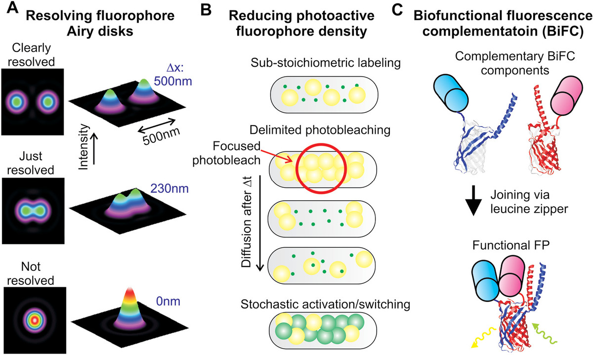
Figure 4.1 Resolving fluorophores. (a) Airy disk intensity functions displayed as false-color heat maps corresponding to two identical fluorophores separated by 500 nm (clearly resolved), 230 nm (just resolved), and 0 nm (not resolved—in fact, located on top of each other). (b) Methods to reduce the density of photoactive fluorophores inside a cell to ensure that the concentration is less than Clim, at which the nearest-neighbor photoactive fluorophore separation is equal to the optical resolution limit. (c) BiFC that uses genetic engineering technology (see Chapter 7) to generate separate halves of a fluorescent protein that only becomes a single-photoactive fluorescence protein when the separate halves are within a few nanometers of each other to permit binding via a leucine zipper.
This indicates that the first-order intensity minimum at an angle a satisfies
(4.2)The Rayleigh criterion for optical resolution states that two PSF images can just be resolved if the peak intensity distribution of one falls on the first-order minimum of the other. The factor of 1.22 comes from the circularity of the aperture; the wavelength λm in propagating through an optical medium of refractive index n is λ/n where λ is the wavelength in a vacuum. Therefore, if f is the focal length of the objective lens, then the distance the optical resolution in terms of displacement along the x axis in the focal plane Δx is
(4.3)This is a modern version of the Abbe equation, with the optical resolution referred to as the Abbe limit. Abbe defined this limit first in 1873 assuming an angular resolution of sin θ = λm/d for a standard rectangular diffraction grating of width d, with the later factor of 1.22 added to account for a circular aperture. An Airy ring diffraction pattern is a circularly symmetrical intensity function with central peak containing ~84% of the intensity, such that multiple outer rings contain the remaining intensity interspaced by zero minima.
The Rayleigh criterion, from the eponymous astronomer, based on observations of stars, which appear to be so close together that they are difficult to resolve by optical imaging, is semiarbitrary in suggesting that two objects could be resolved using circular optics if the central maximum of the Airy ring pattern of one object is in the same position as the first-order minimum of the other, implying the Abbe limit of ~0.61λ/NA. However, there are other suggested resolution criteria that are perfectly reasonable, in that whether or not objects are resolved is as much to do with neural processing of this intensity information in the observer’s brain as it is with physics. One such alternative criterion calls for there being no local dip in intensity between the neighboring Airy disks of two close objects, leading to the Sparrow limit of ~0.47λ/NA. The experimental limit was first estimated quantitatively by the astronomer Dawes, concluding that two similarly bright stars could be just resolved if the dip in intensity between their images was no less than 5%, which is in fact closer to the Sparrow limit than the Rayleigh criterion by ~20%. Note that there is in fact a hard upper limit to optical resolution beyond which no spatial frequencies are propagated (discussed later in this chapter).
In other words, the optical resolution is roughly identical to the PSF width in a vacuum. For visible light emission, the optical resolution limit is thus in the range ~250–300 nm for a high-magnification microscope system, two orders of magnitude larger than the length scale of a typical biomolecule. The z resolution is worse still; the PSF parallel to the optic axis is stretched out by a factor of ~2.5 for high-magnification objective lenses compared to its width in x and y (see Chapter 3). Thus, the optical resolution limits in x, y, and z are at least several hundred nanometers, which could present a problem since many biological processes are characterized by the nanoscale length scale of interacting biomolecules.
4.2.2 Localization Microscopy: The Basics
The most straightforward super-resolution techniques are localization microscopy methods. These involve mathematical fitting of the theoretical PSF, or a sensible approximation to it, to the experimentally measured diffraction-limited intensity obtained from a pixel array detector on a high-sensitivity camera. The intensity centroid (see Chapter 8 for details of the computational algorithms used) is generally the best estimate for the location of the point source emitter (the method is analogous to pinpointing with reasonable confidence where the peak of a mountain is even though the mountain itself is very large). In doing so, the center of the light intensity distribution can be estimated to a very high spatial precision, σx, which is superior to the optical resolution limit. This is often performed using a Gaussian approximation to the analytical PSF (see Thompson et al., 2002):
(4.4)where
- s is the width of the experimentally measured PSF when approximated by a Gaussian function
- a is the edge length of a single pixel on the camera detector multiplied by the magnification between the sample and the image on the camera
- b is the camera detector dark noise (i.e., noise due to the intensity readout process and/or to thermal noise from electrons on the pixel sensor)
- N is the number of photons sampled from the PSF
The distance w between the peak of the Airy ring pattern and a first-order minimum is related to the Gaussian width s by s ≈ 0.34w.
The Gaussian approximation has merits of computational efficiency compared to using the real Airy ring analytical formation for a PSF, but even so is still an excellent model for 2D PSF images in widefield imaging. The aforementioned Thompson approximation results in marginally overoptimistic estimates for localization precision, and interested readers are directed to later modeling (Mortensen et al., 2010), which includes a more complex but realistic treatment.
The spatial precision is dependent on three principal factors: Poisson sampling of photons from the underlying PSF distribution, a pixelation noise due to an observational uncertainty as to where inside a given pixel a detected photon actually arrived, and noise associated with the actual camera detection process. It illustrates that if N is relatively large, then σx varies roughly as s/√N. Under these conditions, σx is clearly less than w (a condition for super-resolution). Including the effects of pixelation and dark noise indicates that if N is greater than ~106 photons, then the spatial precision can in principle be at the level of 1 nm to a few tens of nanometers. A popular application of this method has been called “fluorescence imaging with one nanometer accuracy” (see Park, 2007).
To avoid aliasing due to undersampling of the intensity distribution by the camera, Nyquist theory (also known as Nyquist–Shannon information theory) indicates that the pixel edge length multiplied by the image magnification must be less than w. Equation 4.4 can be used with physically sensible values of s, N, and b to estimate the optimal value of a to minimize σx in other words, to optimize the image magnification on the camera to generate the best spatial precision. Typical optimized values of pixel magnification are in the range 50–100 nm of the sample plane imaged onto each pixel.
The effective photon collection efficiency of a typical high-magnification microscope used for localization microscopy is at best ~10%. Therefore, if one were to achieve a theoretical precision as good as 1 nm, then a fluorescence point source emitter must emit at least ~107 photons. A bright single organic dye molecule imaged under typical conditions of epifluorescence microscopy will emit this number of photons after a duration of ~1 s. This sets a limit on the speed of biological processes, which can be probed at a precision of 1 nm to a few tens of nanometers, typical of super-resolution microscopy. Note, however, that in practice, there is often a short linker between the dye tag and the biomolecule being tracked, so the true spatial precision for the location of the biomolecule is a little worse than that expected from localization fitting theory since it needs to include the additional flexibility of the linker also.
4.2.3 Making the Most Out of a Limited Photon Budget
To investigate faster processes requires dividing up the photon budget of fluorescence emission into smaller sampling windows, which therefore implies a poorer spatial precision unless the photon emission flux is increased. For many fluorophores such as bright organic dyes and QDs, this is feasible, since they operate in a subsaturation regime for photon absorption and therefore their fluorescence output can be increased by simply increasing the excitation intensity. However, several less stable fluorophores are used in biophysical investigations, including fluorescent proteins (FPs), which undergo irreversible photobleaching after emitting at least an order of magnitude fewer photons compared to organic dyes.
For example, green fluorescent protein (GFP) emits only ~106 photons prior to irreversible photobleaching for GFP and so can never achieve a spatial precision to the level of 1 nm in localization microscopy in the typical high-efficiency photon collection microscopes currently available. Some variants of FP, such as yellow FP, (YFP), emit in excess of 107 photons prior to irreversible photobleaching and therefore have potential application for nanoscale imaging. But similarly, there are less stable FPs (a good example is cyan FP [CFP]) that only emit ~105 photons before irreversible photobleaching.
Irreversible photobleaching, primarily due to free radical formation, can be suppressed by chemical means using quenchers. In essence, these are chemicals that mop up free radicals and prevent them from binding to fluorophores and inactivating their ability to fluorescence. The most widely used is based on a combination of the sugar glucose (G) and two enzymes called “glucose oxidase” (GOD) and “catalase” (CAT). The G/GOD/CAT freeradical quencher works through a reaction with molecular oxygen (
where glucose is a substrate for GOD, which transfers electrons in glucose to form a product glucuronic acid (GA), and hydrogen peroxide (H2O2). In a second reaction, CAT transfers electrons from two molecules of hydrogen peroxide to form water and oxygen gas. The downside is that as GA accumulates, the pH of the solution potentially drops, and so strong pH buffers are required to prevent this, though there are some newer quencher systems available that have less effect on pH.
As a rough guide, at video-rate imaging of a typical FP such as GFP, a high-magnification fluorescence microscope optimized for single-molecule localization microscopy can achieve a localization precision in the lateral xy focal plane of a few tens of nanometers, with irreversible photobleaching occurring after 5–10 image frames per GFP, or ~200–400 ms at video-rate sampling. If faster sampling time is required, for example, to overcome motion blurring of the fluorophore in cytoplasmic environments, then detection may need to be more in the range of 1–5 ms per image frame, and so the total duration that a typical FP can be imaged is in the range ~5–50 ms. However, as discussed in the previous section, strobing can be implemented to space out this limited photon emission budget to access longer time scales where appropriate for the biological process under investigation.
4.2.4 Advanced Applications of Localization Microscopy
Localization microscopy super-resolution approaches have been successively applied to multicolor fluorescence imaging in cells, especially dual-color imaging, also known as colocalization microscopy, where one biomolecule of interest is labeled with one-color fluorophore, while a different protein in the same cell is labeled with a different color fluorophore, and the two emission signals from each are split optically on the basis of wavelength to be detected in two separate channels (see Chapter 8 for robust computational methods to determine if two fluorophores are colocalized or not). This has led to a surplus of acronyms for techniques that essentially have the same core physical basis. These include single-molecule high-resolution colocalization that can estimate separations of different colored fluorophores larger than ~10 nm (Warshaw et al., 2005, for the technique’s invention; Churchman et al., 2005, for invention of the acronym). Also, techniques called “single-molecule high-resolution imaging with photobleaching” (Gordon et al., 2004) and “nanometer-localized multiple single-molecule fluorescence microscopy” (Qu et al., 2004) both use photobleaching to localize two nearby fluorophores to a precision of a few nanometers up to a few tens of nanometers. Single-particle tracking localization microscopy (TALM) uses localization microscopy of specifically mobile-tagged proteins (Appelhans et al., 2012).
4.2.5 Limiting Concentrations for Localization Microscopy
Localization microscopy super-resolution techniques are effective if the mean nearest-neighbor separation of fluorophores in the sample is greater than the optical resolution limit, permitting the PSF associated with a single fluorophore to be discriminated from others in solution. Therefore, there is a limiting concentration of fluorescently tagged molecules in a cell that will satisfy this condition. This depends upon the spatial dimensionality of the localization of the biomolecule. For example, it might be 3D in the cell cytoplasm, 2D confined to the cell membrane, or even 1D delimited to a filamentous molecular track. Also, it depends upon the mobility of the molecule in question.
The distribution of nearest-neighbor distances can be modeled precisely mathematically (see Chapter 8); however, to obtain a rough idea of the limiting concentration Clim, we can use the simple arguments previously in this chapter indicating that in the cytoplasm, the mean fluorophore concentration in a typical bacterial cell such as Escherichia coli used is equivalent to ~50–350 molecules per cell, depending on whether they are free to diffuse (low end of the range) or immobile but randomly distributed (high end of the range). In practice, much of a cell contains excluded volumes (such as due to the presence of DNA genetic material), and/or biomolecules may group together in a nonrandom way, so in reality, there may be nontrivial differences from cell to cell and molecule to molecule (see Worked Case Example 4.1).
There are several different types of biomolecules that are expressed in low copy numbers in the cell, some of which, such as transcription factors, regulate the on/off switching of genes, down to only 1–10 per cell in E. coli at any one time, which therefore satisfy the mean nearest-neighbor distance condition to be distinctly detected. However, there are similarly other types of molecules that are expressed at effective mean concentration levels per cell of four or more orders of magnitude beyond this (see Chapter 1), whose concentration therefore results in typical nearest-neighbor separations that are less than the optical resolution limit.
In practice, what often happens is that single fluorescently tagged molecules, often FPs, integrate into molecular machines in living cells. These often have characteristic modular molecular architecture, meaning that a given molecule may be present in multiple copies in a given molecular complex in the machine. These machines have a characteristic length scale of ~5–50 nm, much less than the optical resolution limit, and since the image is a convolution of the PSF for a single fluorophore with the spatial probability function for all such fluorophores in the machine, this results in a very similar albeit marginally wider PSF as a single fluorophore but with an amplitude greater by a factor equal to the number of copies of that fluorophore in the machine.
4.2.6 Substoichiometric Labeling and Delimited Photobleaching
There are several techniques to overcome the nearest-neighbor problem. One of the simplest is to substoichiometrically label the molecular population of interest, for example, adjusting the concentration of fluorescent dyes relative to the biomolecule of interest and reducing the incubation time. This involves labeling just a subpopulation of molecules of a specific type such that the cellular concentration of fluorophore is below Clim. Irreversibly, photobleaching a proportion of fluorophores in a cell with excitation light for a given duration prior to normal localization microscopy analysis can also reduce the concentration of photoactive fluorophore in cell to below Clim (Figure 4.1b).
This method is superior to substoichiometric labeling in that there are not significant numbers of unlabeled molecules of interest in the cell, which would potentially have different physical properties to the tagged molecule such as mobility and rates of insertion into a complex so forth, and also has the advantage of being applicable to cases of genomic FP-fusion labeling. This method has been used to monitor the diffusion of fluorescently labeled proteins in the cell membrane of bacteria using a high-intensity focused laser bleach at one end of the cell to locally bleach a ~1 μm diameter region and then observe fluorescence subsequently at a lower laser intensity. The main issue with both of these approaches is that they produce a dark population of the particular biomolecule that is under investigation, which may well be affecting the experimental measurements but which we cannot detect.
Dynamic biological processes may also be studied using substoichiometric labeling in combination with fluorescent speckle microscopy (see Waterman-Storer et al., 1998). Here, a cellular substructure is substoichiometrically labeled with fluorescent dye (i.e., meaning that not all of the molecules of a particular type being investigated are fluorescently labeled). This results in a speckled appearance in conventional fluorescence imaging, and it has been employed to monitor the kinetics and mobility of individual protein molecules in large molecular structures. The fluorescent speckle generates an identifiable pattern, and movement of the protein assembly as a whole results in the pattern image translating. This can be measured accurately without the need for any computationally intensive fitting algorithms and has been applied to the study of microtubular structures in living cells.
4.2.7 Genetic Engineering Approaches to Increase the Nearest-Neighbor Distance
For FP-labeling experiments, it may be possible to control concentration levels of the fluorophore through the application of inducer chemicals in the cell (see Chapter 7). This is technically challenging to optimize predictably, however. Also, there are issues of deviations from native biological conditions since the concentration of the molecules observed may, in general, be different from their natural levels.
Pairs of putatively interacting proteins can satisfy the Clim condition using a technique called “bifunctional fluorescence complementation” (BiFC). Here, one of the proteins in the pair is labeled with a truncated nonfluorescent part of a FP structure using the same type of genetics technology as for conventional FP labeling. The other protein in the pair is labeled with the complementary remaining part of the FP structure. When the two molecules are within less than roughly a nanometer of each other, the complementary parts of the FP structure can bind together facilitated by short alpha helical attachment made from leucine amino acids that interact strongly to form a leucine zipper motif. In doing so, a fully functional FP is then formed (Figure 4.1c), with a cellular concentration, which may be below Clim even though those of the individual proteins themselves may be above this threshold.
4.2.8 Stochastic Activation and Switching of Fluorophores
Ensuring that the photoactive fluorophore concentration is below Clim can also be achieved through stochastic activation, photoswitching, and blinking of specialized fluorophores.
The techniques of photoactivatable localization microscopy (PALM) (Betzig et al., 2006) are essentially the same in terms of core physics principles as the ones described for fluorescence photoactivatable localization microscopy and stochastic optical reconstruction microscopy (STORM) (Rust et al., 2006). They use photoactivatable or photoswitchable fluorophores to allow a high density of target molecules to be labeled and tracked. Ultraviolet (UV) light is utilized to stochastically either activate a fluorophore from an inactive into a photoactive form, which can be subsequently excited into fluorescence at longer visible light wavelengths, or to switch a fluorophore from, usually, green color emission to red.
Both approaches have been implemented with organic dyes as well as FPs (e.g., photoactivatable GFP [paGFP], and PAmCherry in particular, and photoswitchable proteins such as Eos and variants and mMaple). Both techniques rely on photoconversion to the ultimate fluorescent state being stochastic in nature, allowing only a subpopulation to be present in any given image and therefore increasing the typical nearest-neighbor separation of photoactive fluorophores to above the optical resolution threshold. Over many (>104) repeated activation/imaging cycles, the intensity centroid can be determined to reconstruct the localization of the majority of fluorescently labeled molecules. This generates a super-resolution reconstructed image of a spatially extended subcellular structure.
The principal problems with PALM/STORM techniques are the relatively slow image acquisition time and photodamage effects. Recent faster STORM methods have been developed, which utilize bright organic dyes attached via genetically encoded SNAP-Tags. These permit dual-color 3D dynamic live-cell STORM imaging up to two image frames per second (Jones et al., 2011), but this is still two to three orders of magnitude slower than many dynamic biological processes at the molecular scale. Most samples in PALM/STORM investigations are chemically fixed to minimize sample movement, and therefore, the study of dynamic processes, and of potential photodamage effects, is not relevant. However, the use of UV light to activate and/or switch fluorophores, and of visible excitation light for fluorescence imaging, over several thousand cycles substantially increases concentration of free radicals in cellular samples. This potentially impairs the viability of non-fixed cells.
The phrase time-correlated single-molecule localization microscopy (tcSMLM) is sometimes used to describe the subset of localization microscopy techniques, which render time-resolved information. This is generally from using tracking of positional data, which estimate the peak of the fluorophore’s 2D intensity profile, but other methods also utilize time-dependent differences in photophysical fluorophore properties such fluctuations of brightness and fluorescence lifetimes, which may be applied to multiple fluorescent emitters in a field of view, including super-resolution optical fluctuation imaging (SOFI) (Dertinger et al, 2009) which uses temporal intensity statistics to generate super-resolved image data, and a range of recent algorithms which use statistical analysis of dye brightness fluctuations, for example, Bayesian analysis of bleaching and blinking (3B) (Cox et al, 2012), which can overcome several of the issues associated with high fluorophore density, which straightforward tracking methods can be limited by.
The most widely applied tcSMLM approach uses PALM instrumentation, called time-correlated PALM (tcPALM), in which PALM is used to provided time-resolved information from individual tracks (Cissé et al. 2013). As with normal PALM, only a fraction of the tagged molecules present can be localized so this does not render a definitive estimate for the total number of molecules present of that particular type but does yield quantitative details of their dynamics from the subset that are labeled and detected once stochastically activated. Here, for example, PALM can image a region of a cell expected to have a high concentration of molecular clusters comprising a specific protein labeled with a photoactivatable dye, and then a time-series is acquired recording the time from the start of activation at which every track is subsequently detected. The peak time from this distribution, inferred from many such fields of view form different cells, is then used as a characteristic arrival time for that protein into a molecular complex, which can then be compared against other estimates in which the system is perturbed in some way at which characteristic time for fluorophore to be detected time, and which can be a very tool to understand the reactions that occur in the cluster assembly process.
4.2.9 Stochastic Blinking
Reversible photobleaching of fluorophores, or blinking, can also be utilized (for a good review of the fluorophore photophysics, see Ha and Tinnefeld, 2012). The physical mechanism of blinking is heterogeneous, in that several potential photophysical mechanisms can lead to the appearance of reversible photobleaching. Occupancy of the triplet state, or triplet blinking, is one of such; however, the triplet state lifetime is ~10−6 s, which is too small to account for observed blinking in fluorescence imaging with a sampling time window of ~10−3 s and above. Redox blinking is another possible mechanism in that an excited electron is removed (one of the definitions of oxidation), which induces a dark state that is transient up until the time that a new electron is elevated to the excited state energy level. However, many different fluorophores also appear to have nonredox photochemical mechanisms to generate blinking.
The stochastic nature of photoblinking can be carefully selected using different chemical redox conditions but also, in some cases, through a dependence of the blinking kinetics on the excitation light intensity. High-intensity light, in excess of several kW cm−2, can give rise to several reversible blinking cycles before succumbing to irreversible photobleaching. This reduces the local concentration of photoactive fluorophores in any given image frame, facilitating super-resolution localization microscopy. This technique has been applied to living bacterial cells to map out DNA binding proteins using YFP (Lee et al., 2011).
An alternative stochastic super-resolution imaging method is called “point accumulation for imaging in nanoscale topography.” Here, fluorescence imaging is performed using diffusing fluorophore-tagged biomolecules, which are known to interact only transiently with the sample. This method is relatively straightforward to implement compared to PALM/STORM. This method has several variants, for example, it has also been adapted to a membrane-localized protein to generate super-resolution cell membrane features in a technique described as super-resolution by power-dependent active intermittency and points accumulation for imaging in nanoscale topography (SPRAIPAINT) (Lew et al., 2011).
Dye blinking of organic dyes has also been utilized in a technique called “blinking assisted localization microscopy” (Burnette et al., 2011). This should not be confused with binding-activated localization microscopy, which utilizes a fluorescence enhancement of a dye when bound to certain cellular structures such as nucleic acids compared to being free in solution, which can be optimized such that the typical nearest-neighbor distance is greater than the optical resolution limit (Schoen et al., 2011). Potential advantages over PALM/STORM of blinking localization microscopy are that the sampling time scales are faster and also that there is less photodamage to living cells in avoiding the more damaging shorter wavelength used in UV-based activation.
Improvements to localization microscopy precision can be made using prior information concerning the photophysics of the dyes, resulting in a hybrid technique of analytical inference with standard localization tools such as PALM/STORM. Bayesian analysis is an ideal approach in this regard (discussed fully in Chapter 8). This can be applied to photoblinking and photobleaching observations trained on prior knowledge of both. Bayesian blinking and bleaching microscopy (3B microscopy) analyzes data in which many overlapping fluorophores undergo both bleaching and blinking events to generate spatial localization information at enhanced resolution. It uses a hidden Markov model (HMM). An HMM assumes that the underlying process is a Markov process (meaning future states in the system depend only on the present state and not on the sequence of events that preceded it, i.e., there is no memory effect) but with unobserved (hidden) states and is often used in Bayesian statistical analysis (see Chapter 8). It enables information to be obtained that would be impossible to extract with standard localization microscopy methods.
The general issue of photodamage with fluorescence imaging techniques should be viewed in the following context:
- All imaging of live cells with fluorescence (and many other modalities) is potentially damaging, for example, fast confocal scanners often kill a muscle cell in seconds. That is, however, acceptable, for certain experiments where we are looking at fast biological processes (e.g., a few milliseconds) and the mindful biologist builds in careful control experiments to make sure they can put limits on these effects.
- The degree of damage seen is likely closely connected to the amount of information derived but can be reduced if light dosage is reduced using hybrid approaches such as 3B microscopy. Some spatial resolution is inevitably sacrificed for time resolution and damage reduction—nothing is for free.
- Many dark molecules in photoactivating super-resolution methods greatly reduce absorption in the sample, and the UV exposure to photoactivate is generally very low.
4.2.10 Reshaping the PSF
The Abbe diffraction limit for optical resolution can also be broken using techniques that reduce the size of the PSF. One of these is 4Pi microscopy (Hell and Stelzer, 1992). Here, the sample is illuminated with excitation light from above and below using matched high NA objective lenses, and the name of the technique suggests an aspiration to capture all photons emitted from all directions (i.e., 4π steradians). However, in reality, the capture solid angle is less than this. The technique improves the axial resolution by a factor of ~5 to more 100–150 nm, generating an almost spherical focal volume six times smaller than confocal imaging.
Stimulated-emission depletion microscopy (STED) (see Hell and Wichmann, 1994) and adapted techniques called “ground state depletion,” “saturated structured illumination microscopy” (SSIM), and “reversible saturable optical fluorescence transitions” microscopy all reduce the size of the excitation volume by causing depletion of fluorescence emissions from the outer regions of the usual Airy ring PSF pattern. Although these techniques began as in vitro super-resolution methods, typically to investigate the aspect of cytoskeletal structure (to this day, the ability to resolve single-microtubule filaments of a few tens of nanometer width in a tightly packed filament is treated as a benchmark of the technique), they have also now developed into powerful cellular imaging tools.
In STED, this reduction in laser excitation volume is achieved using a second stimulated emission laser beam in addition to an excitation beam, which is shaped like a donut in the focal plane with a central intensity minimum of width ~200 nm. This annulus intensity function can be generated using two offset beams or by phase modulation optics (Figure 4.2a).
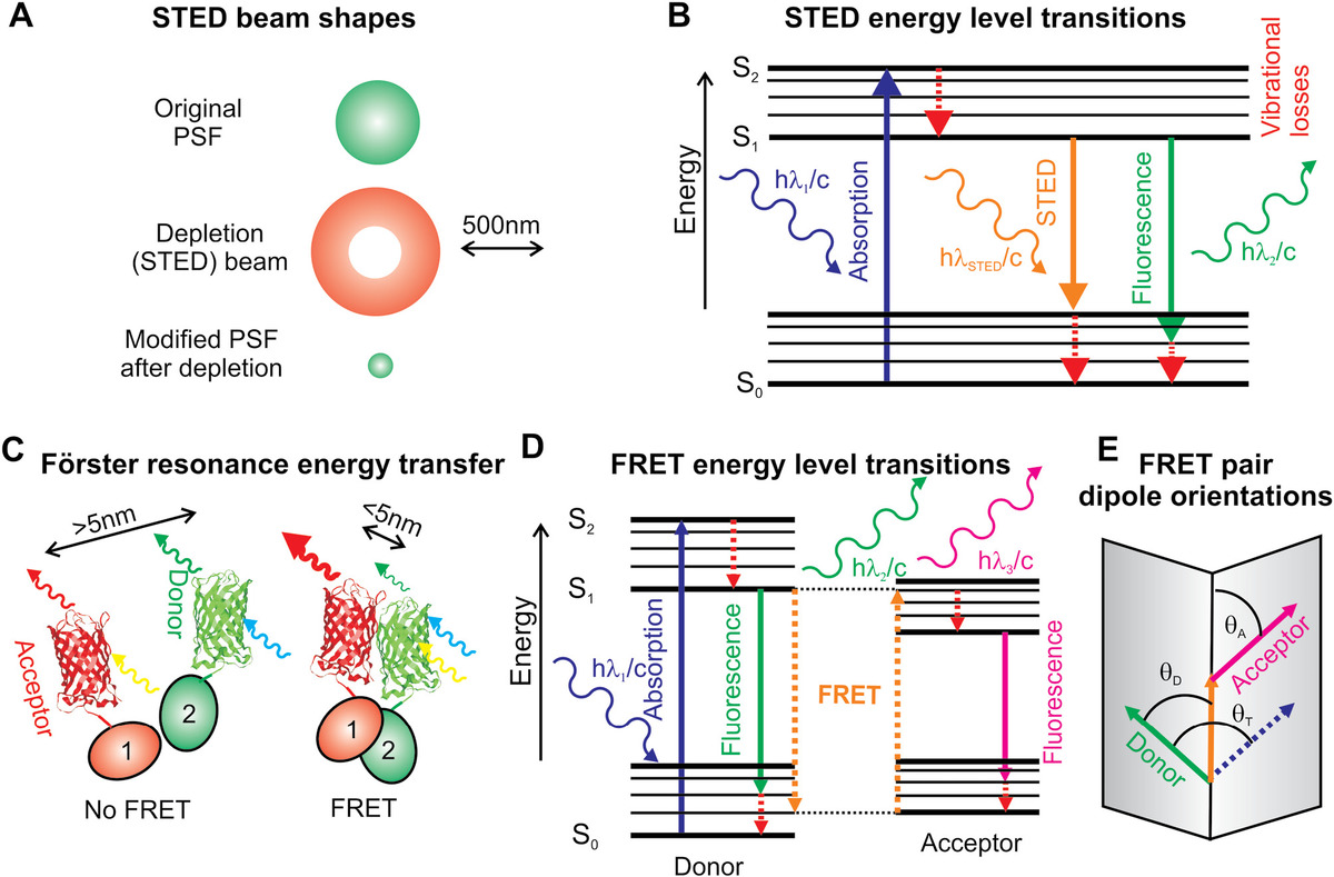
Figure 4.2 Stimulated-emission depletion microscopy (STED) and Förster resonance energy transfer (FRET). (a) Relative sizes and shapes of STED depletion beam and original PSF of a fluorophore; the donut-shaped depletion beam stimulates emission depletion from the fluorophore to generate a much smaller point spread function intensity volume, with (b) the associated Jablonski energy level diagram indicated. (c) Schematic depiction of FRET, here, indicated between a donor and acceptor fluorescent protein, which are excited by short and long light wavelengths respectively, with (d) associated Jablonski energy level diagram and (e) schematic indicating the relative orientation of the donor–acceptor fluorophore electric dipole moment axes; each respective electric dipole axis lies in a one of two planes separated by angle θT, and these two planes intersect at a line defined by arrow indicated that makes angles θA and θD with the acceptor and donor electric dipole axes, respectively.
This beam has a longer wavelength than the laser excitation beam and stimulates emission from the fluorescence excited state (Figure 4.2b), resulting in the depletion of the excited state in the high-intensity region of the donut, but a nondepleted central region whose volume is much smaller than the original PSF. In STED, it is now standard to reduce the width w of the excitation volume in the sample plane to <100 nm, which, assuming an objective lens of numerical aperture NA, is given by
(4.6)where
- λ is the depletion beam wavelength with saturating intensity Is (intensity needed to reduce fluorescence of the excited state by a factor of 2)
- I is the excitation intensity at the center of the donut
For large I, there is an ~1/√I, dependence on w, so w could in principle be made arbitrarily small. A limiting factor here is irreversible photobleaching of the fluorophores used, resulting in a few tens of nanometers for most applications at present. Due to the absence of shorter wavelength UV activation, STED excitation can penetrate deeper with less scatter into large cells, which has some advantages over PALM/STORM. Also, maximum image sampling rates are typically higher than for PALM/STORM at a few tens of frames per second currently higher for STED compared to a few per second for PALM/STORM. However, there are potentially greater issues of photodamage with STED due to the high intensity of the depletion beam.
Minimal photon FLUX (MinFlux) microscopy (Balzarotti et al 2016) is a related super-resolution tool that combines SMLM and STED while using fewer fluorescence photons but enabling higher spatial and time resolution. In MinFlux, the STED donut-shaped bead is steered to map onto the molecular position itself while eliciting minimum fluorenscent photon emissions from the dye molecule. In Minflux, the donut beam is scanned across a sample to minimally acquire emission data sufficient to estimate roughly where a dye molecule is by using probabilistic triangulation criteria based on the brightness of the fluorescence and the spatial position of the donut beam. This estimate is then used to fine-tune the position of the donut beam to center it over the dye by shifting the beam over an area of length scale, L ~50 nm, and then STED as normal is performed. However, since the center of the donut beam, the zero-excitation intensity region, is now roughly colocalized with the dye position, then the dye molecule subsequently emits relatively low numbers of fluorescent photons.
The spatial precision, instead of scaling with ~λ/(NA√N) as suggested by Equation 4.6 scales as ~~L/√N. This results in a spatial precision of 1–3 nm for as few as a ~500 emitted photons but can be made significantly smaller by reducing L to nanoscale levels, thus allowing for true nanoscale spatial resolution but with substantively longer duration acquisitions while minimizing photobleaching of the dyes. Also, since steering of the donut beam uses rapid piezoelectric and electro-optical control, the time resolution for 2D imaging can be as low as a few hundred microseconds, hence rapid enough to enable single-molecule dye diffusion to be tracked unblurred in the cytoplasm of live cells, with tracking really then limited only by photoblinking of the dyes themselves.
Variants of the technique enabling multicolor 3D MinFlux imaging now exist (e.g. using a “z-donut,” i.e., a 3D shell-intensity depletion beam volume). At the time of writing, basic SMLM bespoke microscopy can be implemented for as a little as few tens of thousands of USD with higher throughput compared to MinFlux, whereas the equivalent cost for a basic MinFlux system is roughly an order of magnitude greater. Although promising developments are being made with structured illumination to increase MinFlux throughput, the main barrier to its more widespread application is arguably cost.
4.2.11 Patterned Illumination Microscopy
Structured illumination microscopy (SIM), also known as patterned illumination microscopy, is a super-resolution method that utilizes the Moiré pattern interference fringes generated in the focal plane using a spatially patterned illumination (Gustafsson, 2000). Moiré fringes are equivalent to a beat pattern. When measurements are made in the so-called reciprocal space or frequency space in the Fourier transform of the image, smaller length scale features in the sample are manifested at higher spatial frequencies, such that the smallest resolvable feature using conventional diffraction-limited microscopy has the highest spatial frequency. In generating a beat pattern, spatial frequencies above this resolution threshold are translated to lower values in frequency space. On performing an inverse Fourier transform, this therefore reveals spatial features that would normally be smaller than the optical resolution limit. In practice, the fringe pattern is rotated in the focal plane at multiple orientations (three orientations separated by 120° is typical) to obtain resolution enhancement across the full lateral plane. The actual pattern itself is removed from the imaging by filtering in frequency space; however, unavoidable artifacts of the pattern lines do occur, which can result in embarrassing overinterpretation of cellular data if careful controls are not performed.
The spatial resolution enhancement in standard SIM relies on a linear increase in spatial frequency due to the sum of spatial frequencies from the sample and pattern illumination. The latter is diffraction-limited and so the maximum possible enhancement factor for spatial resolution is 2. But, if the rate of fluorescence emission is nonlinear with excitation intensity (e.g., approaching very high intensities close to photon absorption saturation of the fluorophore), then the effective illumination pattern may contain harmonics with spatial frequencies that are integer multiples of the fundamental spatial frequency from the pattern illumination and can therefore generate greater enhancement in spatial resolution. This has been utilized in nonlinear SIM techniques called “saturated pattern excitation microscopy” and SSIM, which can generate a spatial resolution of a few tens of nanometers. The laser excitation intensities required are high, and therefore, sample photodamage is an issue, and the imaging speeds are currently still low at a maximum of tens of frames per second.
4.2.12 Near-Field Excitation
Optical effects that occur over distances less than a few wavelengths are described as near-field, which means that the light does not encounter significant diffraction effects and so the optical resolution is better than that suggested by the Abbe diffraction limit. This is utilized in scanning near-field optical microscopy (SNOM or NSOM) (Hecht et al., 2000). This often involves scanning a thin optical fiber across a fluorescently labeled sample with excitation and emission light conveyed via the same fiber. The vertical distance from sample to fiber tip is kept constant at less than a wavelength of the emitted light. The lateral spatial resolution is limited by the diameter of the optical fiber itself (~20 nm), but the axial resolution is limited by scanning reliability (~5 nm). Scanning is generally slow (several seconds to acquire an image), and imaging is limited to topographically accessible features on the sample (i.e., surfaces).
However, samples can also be imaged in SNOM using other modes beyond simply capturing reflected and/or emitted light. For example, many of SNOM’s applications use transmission mode with the illumination external to the fiber. These are either oblique above the sample for reflection, or from underneath a thin transparent sample for transmission. The fiber then collects the transmitted/reflected light after it interacts with the sample.
An important point to consider is the long time taken to acquire data using SNOM. SNOM takes several tens of minutes to acquire a single image at high pixel density, an order of magnitude longer than alternative scanning probe methods such as atomic force microscopy (AFM) for the equivalent sample area (see Chapter 6). The high spatial resolution of ~20 nm that results is a great advantage with the technique, though the poor time resolution is a significant drawback with regard to monitoring the dynamic biological processes. Fluorescent labeling of samples is not always necessary for SNOM, for example, the latest developments use label-free methods employing an infrared (IR)-SNOM with tuneable IR light source.
Near-field fluorescence excitation fields can be generated from photonic waveguides. Narrow waveguides are typically manufactured out of etched silicon to generate channels of width ~100 nm. A laser beam propagated through the silicon generates an evanescent excitation field in much the same wave as for total internal reflection fluorescence (TIRF) microscopy (see Chapter 3). Solutions containing fluorescently labeled biomolecules can be flowed through a channel and excited by the evanescent near-field. Many flow channels can be manufactured in parallel, with surfaces precoated by antibodies, which then recognize different biomolecules, and this therefore is a mechanism to enable biosensing. Recent improvements to the sensitivity of these optical microcavities utilize the whispering gallery mode in which an optically guided wave is recirculated in silicon crystal of a circular shape to enhance the sensitivity of detection in the evanescent near-field to the single-molecule level (Vollmer and Arnold, 2008).
4.2.13 Super-Resolution in 3D and 4D
Localization microscopy methods are routinely applied to 2D tracking of a variety of fluorophore-labeled biomolecules in live cells. However, to obtain 3D tracking information presents more challenges, due in part to mobile particles diffusing from a standard microscope’s depth of field faster than refocusing can be applied, and so they simply go out of focus and cannot be tracked further. This, coupled with the normal PSF image of a fluorophore within the depth of field, results in relative insensitivity to z displacement. With improvements in cytoplasmic imaging techniques of cellular samples, there is a motivation to probe biological processes deeper inside relatively large cells and thus a requirement for developing 3D tracking methods. (Note that these techniques are sometimes referred to as “4D,” since they generate information from three orthogonal spatial dimensions, in addition to the dimension of time.)
There are three broad categories of 3D tracking techniques. Multiplane imaging, most commonly manifested as biplane imaging, splits fluorescence emissions from a tracked particle to two or more different image planes in which each has a slight focal displacement offset. This means that the particle will come into sharp focus on each plane at different relative distances from the lateral focal plane of the sample. In its most common configuration of just two separate image planes, this can be achieved by forming the two displaced images onto separate halves of the same camera detector. Standard 2D localization fitting algorithms can then be applied to each image to measure the xy localizations of the particle as usual and also estimate the z value from extrapolation of the pixel intensity information compared to a reference of an in-focus image of, for example, a surface-immobilized fluorophore. This technique works well for bright fluorophores, but in having to split the fluorescence photon budget between different images, the localization precision is accordingly reduced by a factor of ~√2. Also, although the real PSF of a fluorescence imaging system shows in general some asymmetry in z, this asymmetry is normally only noticeable at a few hundred nanometers or more away from the focal plane. Therefore, unless the different focal planes are configured to be separated by at least this threshold distance, there is some uncertainty as to whether a tracked particle very close to the focal plane is diffusing above or below it or, in having to separate the focal planes by relatively large distances inevitably reduces the sensitivity in z at intermediate smaller z values. Similarly, there can be reductions in z sensitivity with this method if separate tracked spots are relatively close to each other in z so as to be difficult to distinguish (in practice, the threshold separation is the axial optical resolution limit that is ~2.5 times that of the lateral optical resolution limit, close to 1 μm, which is the length scale of some small cells such as bacteria and cell organelles in eukaryotes such as nuclei).
Astigmatism imaging is a popular alternative method to multiplane microscopy, which is relatively easy to implement. Here, a long focal length cylindrical lens is introduced in the optical pathway between the sample and the camera detector to generate an image of tracked particles on the camera. The cylindrical lens has intrinsic astigmatism, meaning that it has marginally different focal lengths corresponding to the x-axis and y-axis. This results in fluorophores above or below the xy focal plane having an asymmetric PSF image on the camera, such that fluorescence intensity appears to be stretched parallel to either the x- or y-axis depending upon whether the fluorophore is above or below the focal plane and the relative geometry of the cylindrical lens and the camera.
Measuring the separate Gaussian widths in x and y of such a fluorophore image can thus be used as a sensitive metric for z, if employed in combination with prior calibration data from surface-immobilized fluorophores at well-defined heights from the focal plane. The rate of change of each Gaussian width with respect to changes in z when the Gaussian width is minimum is zero (this is the condition when the fluorophore image is in focus with respect that the appropriate axis of x or y). What is normally done therefore is to toggle between using the x and y widths for the best metric of z, at different z, in order to span the largest possible z range for an accurate output prediction of z. The main issues with the astigmatism method are that the localization precision in z is worse than that in x and y by a factor of ~1.5 and also that the maximum range in z, when using a typical high-magnification microscope optimized for localization microscopy, is roughly ±1 μm.
Corkscrew PSF methods, the most common of which is the double-helical PSF (DH-PSF) approach, can be used to generate z information for fluorophore localization. These techniques use phase modulation optics to generate helical, or in the case of the DH-PSF method, double-helical-shaped PSFvolumes in the vicinity of the sample plane. The helical axis is set parallel to the optic (z) axis such that when a fluorophore is above or below the focal plane, the fluorophore image rotates around this central axis. In the case of DH-PSF imaging, there appear to be two fluorescent spots per fluorophore, which rotate around the central axis with changes in z. In this instance, x and y can also be determined for the fluorophore localization as the mean from the two separate intensity centroid values determined for each separate spot in a pair.
This method has a downside of requiring more expensive phase modulation optics in the form of either a fixed phase modulation plate placed in a conjugate image plane to the back aperture of the objective lens (conjugate to the Fourier transformation plane of the sample image) or a spatial light modulator (SLM) consisting of an array of electrically programmable LCD crystals, which can induce controllable levels of phase retardation across a beam profile. However, the precision in z localization is more than twice as good as the other two competing methods of multiplane and astigmatism imaging (see Badieirostami et al., 2010). A downside is that all multilobe-type methods have a larger in-plane extent, which further reduces the density of active markers that can be imaged without overlap, which can present a real issue in the case of intermediate-high copy number systems (i.e., where the concentrations of fluorescently labeled biomolecules is reasonably high).
4.3 Förster Resonance Energy Transfer
Förster resonance energy transfer (FRET) is a nonlinear optical technique that operates over length scales, which are approximately two orders of magnitude smaller than the optical resolution limit. Thus it be considered a super-resolution technique, but is discussed as a separate section due to its specific utility in probing molecular interactions in biology. Although there is a significant body of literature now concerning the application of FRET in light microscopy investigations, the experimental technique was developed originally from bulk ensemble in vitro assays not using light microscopy. FRET still has enormous applications in that context. Changes to FRET efficiency values can be measured in a suitable fluorimeter, which contains two-color detector channels, one for the so-called donor and the other for acceptor fluorescence emissions. However, the cutting edge of FRET technology uses optical microscopy to probe putative molecular interactions at a single-molecule level.
4.3.1 Efficiency of FRET
This is a nonradiative energy transfer between a donor and acceptor molecule over a length scale of ~1–10 nm, which occurs due to overlapping of the electronic molecular orbitals in both spatial localization and in transition energy level gaps. Often, in practice, as an experimental technique, FRET utilizes fluorescent molecules for donor and acceptor whose electronic energy levels for excitation and emission overlap significantly, and so the term fluorescent energy resonance transfer is sometimes applied, though the physical process of FRET in itself does not necessarily require fluorescence. The length scale of operation of FRET is comparable to that of many biomolecules and molecular machines and so can be used as a metric for molecular interaction between two different molecules if one is labeled with a donor and the other with an appropriate acceptor molecule.
In FRET, the donor fluorophore emits at a lower peak wavelength than the acceptor fluorophore. Resonance transfer of energy between the two is therefore manifest as a small reduction in fluorescence emission intensity from the donor, and a small increase in fluorescence emission intensity of the acceptor (Figure 4.2c and d). The length scale of energy transfer is embodied in the Förster radius, R0, which is the distance separation that yields a FRET efficiency of exactly 0.5. The efficiency ε of the energy transfer as a function of the length separation R of the donor–acceptor pair is characterized by
(4.7)The constant kFRET is the rate of energy transfer from donor to acceptor by FRET, whereas the summed parameters Σki are the energy transfer rates from the donor of all energy transfer processes, which include FRET and radiative processes plus various non-FRET and nonradiative processes (Σki). With no acceptor, a donor transfers energy at rate (kradiative + Σki), and so the mean donor lifetime TD is equal to 1/(kradiative + Σki). With an acceptor present, FRET occurs at a rate kFRET such that the donor lifetime τDA is then equal to (R0/R)6/kFRET, indicating that ε = 1 − τDA/τD.
We can also write ε = 1 − IDA/ID where IDA and ID are the total fluorescence emission intensities of the donor in the presence and the absence of the acceptor, respectively; in practice, the intensity values are those measured through an emission filter window close to the emission peak of the donor fluorophore in question. Similarly, we can say that ε = (IAD − IA)/IA where IAD and IA are the total fluorescence emission intensities of the acceptor in the presence and the absence of the donor, respectively. These formulations assume that there is minimal fluorophore cross talk between the two excitation lasers used for the acceptor and donor (i.e., that the donor is not significantly excited by the acceptor laser, and the acceptor is not significantly excited by the donor laser). Also, that there is minimal bleed-through between the fluorescence emissions of each fluorophore between the two detector emission channels. A simpler formulation involves the relative FRET efficiency used in ratiometric FRET, of εrel = IA/(IA + ID) with IA and ID being the total fluorescence intensities for acceptor and donor, respectively, following excitation of just the donor. However, if the acceptor and donor emission spectra overlap, then this mixed spectrum must be decomposed into the separate component spectra to accurately measure IA and ID, which is often nontrivial. Rarely, one can equate εrel to the actual FRET efficiency (ε) in the case of minimal laser/fluorophore cross talk, in practice, though converting εrel to the actual FRET efficiency (ε) usually requires two correction factors of the contribution from direct acceptor excitation to IA and the ratio between the donor and the acceptor fluorescence emission quantum yields. Additionally, corrections may be needed to account for any fluorescence bleed-through between the acceptor and donor detector channels.
Note that sometimes a FRET pair can actually consist of a dye molecule and a nearby quencher molecule, instead of a donor and acceptor molecule. Here, the distance dependence between the dye and quencher is the same as that of a donor and acceptor molecule since the mechanism of nonradiative energy transfer is the same. However, the quencher does not emit fluorescence, and so the drop in normalized intensity of a dye molecule undergoing quenching is 1 − ε.
4.3.2 Förster Radius and the Kappa-Squared Orientation Factor
The Förster radius R0 is given by a complex relation of photophysical factors:
(4.8)where
- QD is the quantum yield of the donor in the absence of the acceptor
- κ2 is the dipole orientation factor
- n is the refractive index of the medium (usually of water, ~1.33)
- NA is the Avogadro’s number
- the integral term in the numerator is for the spectral overlap integral such that fD is the donor emission spectrum (with the integral in the denominator normalizing this)
- εA is the wavelength-dependent molar extinction coefficient or molar absorptivity of the acceptor
Typical values of R0 for FRET pairs are in the range 3–6 nm. The R6 dependence on ε results in a highly sensitive response with distance changes. For example, for R < 5 nm, the FRET efficiency ε is typically 0.5–1, but for R > 5 nm, ε falls steeply toward zero. Thus, the technique is very good for determining putative molecular interaction. The κ2 factor is given by
(4.9)where angles θT, θA, and θD are relative orientation angles between the acceptor and donor, defined in Figure 4.2e. The κ2 factor can in theory vary from 0 (transition dipole moments are perpendicular) to 4 (transition dipole moments are collinear), whereas parallel transition dipole moments generate a κ2 of exactly 1. FRET donor–acceptor fluorophore pairs that rotate purely isotropically have an expected κ2 of precisely 2/3. However, care must be taken not to simply assume this isotropic condition. The condition is only true if the rotational correlation time for both the donor and acceptor fluorophores is significantly less than the sampling time scale in a given experiment. Typical rotational correlation times scales are ~10−9 s, and so for fluorescence imaging experiments where the sampling times are 10−2 to 10−3 s, the assumption is valid, though for fast nonimaging methods such as confocal fluorescence detection and fluorescence correlation spectroscopy (FCS) sampling may be over a ~10−6 time scale or faster and then the assumption may no longer be valid. An implication of anisotropic fluorophore behavior is that an observed change in FRET efficiency could be erroneously interpreted as a change in donor–acceptor distance when in fact it might just be a relative orientation change between their respective dipole moments.
4.3.3 Single-Molecule FRET
FRET is an enormously valuable tool for identifying putative molecular interactions between biomolecules, as we discussed for the FLIM–FRET technique previously (see Chapter 3). But using light microscopy directly in nonscanning imaging methods enables powerful single-molecule FRET (smFRET) techniques to be applied to addressing several biological questions in vitro (for a practical overview see Roy et al., 2008). The first smFRET biophysical investigation actually used near-field excitation (Ha et al., 1996), discussed later in this chapter. However, more frequently today, smFRET involves diffraction-limited far-field light microscopy with fluorescence detection of both the donor and accept or fluorophore in separate color channels of high-sensitivity fluorescence microscope (see Worked Case Example 4.2). The majority of smFRET studies to date use organic dyes, for example, a common FRET pair being variants of a Cy3 (green) donor and Cy5 (red) acceptor, but the technique has also been applied to QD and FP pairs (see Miyawaki et al., 1997).
The use of organic fluorophore FRET pairs comes with the problem that the chemical binding efficiency to a biomolecule is never 100%, and so there is a subpopulation of unlabeled “dark” molecules. Also, even when both fluorophores in the FRET pair have bound successively, there may be a subpopulation that are photoinactive, for example, due to free radical damage. Again, these “dark” molecules will not generate a FRET response and may falsely indicate the absence of molecular interaction.
Since the emission spectrum of organic dye fluorophores is a continuum, there is a risk of bleed-through of each dye signal into the other’s respective detector channel, which is difficult to distinguish from genuine FRET unless meticulous control experiments are performed. These issues are largely overcome by alternating laser excitation (ALEX) (Kapanidis et al., 2005). Here, donor and acceptor fluorophores are excited in alternation with respective fluorescence emission detection synchronized to excitation.
One of the most common approaches for using smFRET is with confocal microscope excitation in vitro. Here, interacting components are free to diffuse in aqueous solution in and out of the confocal excitation volume. The ~10−6 m length scale of the confocal volume sets a low upper limit on the time scale for observing a molecular interaction by FRET since the interacting pair diffuses over this length scale in typically a few tens of milliseconds.
An approach taken to increase the measurement time is to confine interacting molecules either through tethering to a surface (Ha et al., 2002) or confinement inside a lipid nanovesicle immobilized to a microscope slide (Benitez et al., 2002). This latter method exhibits less interaction with surface forces from the slide. These methods enable continuous smFRET observations to be made over a time scale of tens of seconds.
A significant disadvantage of smFRET is its very limited application for FP fusion systems. Although certain paired combinations of FPs have reasonable spectral overlap (e.g., CFP/YFP for blue/yellow and GFP/mCherry for green/red), R0 values are typically ~6 nm, but since the FPs themselves have a length scale of a few nanometers, this means that only FRET efficiency values of ~0.5 or less can be measured since the FPs cannot get any closer to each other due to their β-barrel structure. In this regime, it is less sensitive as a molecular ruler compared to using smaller, brighter organic dye pairs, which can monitor nanoscale conformational changes.
A promising development in smFRET has been its application in structural determination of biomolecules. Two-color FRET can be used to monitor the displacement changes involved between two sites of a molecule in conformational changes, for example, during power stroke mechanisms of several molecular machines or the dynamics of protein binding and folding. It is also possible to use more than two FRET dyes in the same sample to permit FRET efficiency measurements to be made between three or more different types of dye molecule. This permits triangulation of the 3D position of the dye molecule. These data can be mapped onto atomic level structural information where available to provide a complementary picture of time-resolved changes to molecular structures.
4.4 Fluorescence Correlation Spectroscopy
Fluorescence correlation spectroscopy (FCS) is a technique in which fluorescently labeled molecules are detected as they diffuse through a confocal laser excitation volume, which generates a pulse of fluorescence emission prior to diffusing out of the confocal volume. The time correlation in detected emission pulses is a measure of fluorophore concentration and rate of diffusion (Magde et al., 1972). FCS is used mainly in vitro but has been recently also applied to generate fluorescence correlation maps of single cells.
4.4.1 Determining the Autocorrelation of Fluorescence Data
FCS is a hybrid technique between ensemble averaging and single-molecule detection. In principle, the method is an ensemble average tool since the analysis requires a distribution of dwell times to be measured from the diffusion of many molecules through the confocal volume. However, each individual pulse of fluorescence intensity is in general due to a single molecule. Therefore, FCS is also a single-molecule technique.
The optical setup is essentially identical to that for confocal microscopy. However, there is an additional fast real-time acquisition card attached to the fluorescence detector output that can sample intensity fluctuation data at tens of MHz to calculate an autocorrelation function, IAuto. This is a measure of the correlation in time t of the pulses with intensity I:
(4.10)where
- the parameter t′ is an equivalent time interval value
If the intensity fluctuations all arise solely from local concentration fluctuations δC that are within the volume V of the confocal laser excitation volume, then
(4.12)where
- r is the displacement of a given fluorophore from the center of the confocal volume
- P is the PSF
- I1 is the effective intensity due to just a single fluorophore
For normal confocal illumination FCS, the PSF can be modeled as a 3D Gaussian volume (see Chapter 3):
(4.13)where wxy and wz are the standard deviation widths in the xy plane and parallel to the optical axis (z), respectively. The normalized autocorrelation function can be written then as
(4.14)This therefore can be rewritten as
(4.15)The displacement of a fluorophore as a function of time can be modeled easily for the case of Brownian diffusion (see Equation 2.12), to generate an estimate for the number density autocorrelation term
An important result from this emerges at the zero time interval value for the autocorrelation intensity function, which then approximates to 1/V〈C〉, or 1/〈N〉, where 〈N〉 is the mean (time averaged) number of fluorophores in the confocal volume. The full form of the autocorrelation function for one type of molecule diffusing in three spatial dimensions through a roughly Gaussian confocal volume with anomalous diffusion can be modeled as Im:
(4.17)Fitting experimental data IAuto with model Im yields estimates for parameters Im(0) (simply the intensity due to the mean number of diffusing molecules inside the confocal volume), I(∞) (which is often equated to zero), τ, and α. The parameter a is the anomalous diffusion coefficient. For diffusion in n spatial dimensions with effective diffusion coefficient D, the general equation relating the mean squared displacement 〈R2〉 after a time t for a particle exhibiting normal or Brownian diffusion is given by Equation 2.12, namely, 〈R2〉 = 2nDt. However, in the more general case of anomalous diffusion, the relation is
(4.18)The anomalous diffusion coefficient varies in the range 0–1 such that 1 represents free Brownian diffusion. The microenvironment inside a cell is often crowded (certain parts of the cell membrane have a protein crowding density up to ~40%), which results in hindered mobility termed anomalous or subdiffusion. A “typical” mean value of a inside a cell is 0.7–0.8, but there is significant local variability across different regions of the cell.
The time parameter τ in Equation 4.17 is the mean “on” time for a detected pulse. This can be approximated as the time taken to diffuse in the 2D focal plane, a mean squared distance, which is equivalent to the lateral width w of the confocal volume (the full PSF width equivalent to twice the Abbe limit of Equation 4.3, or ~400–600 nm), indicating
(4.19)Thus, by using the value of τ determined from the autocorrelation fit to the experimental data, the translational diffusion coefficient D can be calculated.
4.4.2 FCS on Mixed Molecule Samples
If more than one type of diffusing molecule is present (polydisperse diffusion), then the autocorrelation function is the sum of the individual autocorrelation functions for the separate diffusing molecule types. However, the main weakness of FCS is its relative insensitivity to changes in molecular weight, Mw. Different types of biomolecules can differ relatively marginally in terms of Mw; however, the “on” time τ scales approximately with the frictional drag of the molecule, roughly as the effective Stokes radius, which scales broadly as
FCS can also be used to measure molecular interactions between molecules. Putatively, interacting molecules are labeled using different colored fluorophores, mostly dual-color labeling with two-color detector channels to monitor interacting pairs of molecules. A variant of standard FCS called “fluorescence cross-correlation spectroscopy” can then be applied. A modification of this technique uses dual-color labeling but employing just one detector channel, which captures intensity only when the two separately labeled molecules are close enough to be interacting, known as FRET-FCS.
4.4.3 FCS on More Complex Samples
FCS can also be performed on live-cell samples. By scanning the sample through the confocal volume, FCS can generate a 2D image map of mobility parameters across a sample. This has been utilized to measure the variation in diffusion coefficient across different regions of large living cells. As with scanning confocal microscopy, the scanning speed is a limiting factor. However, these constraints can be overcome significantly by using a spinning-disk system. FCS measurements can also be combined with simultaneous topography imaging using AFM (see Chapter 6). For example, it is possible to monitor the formation and dynamics of putative lipid rafts (see Chapter 2) in artificial lipid bilayers using such approaches (Chiantia, 2007).
4.5 Light Microscopy of Deep or Thick Samples
Although much insight can be gained from light microscopy investigations in vitro, and on single cells or thin multicellular samples, ultimately certain biological questions can only be addressed inside thicker tissues, for example, to explore specific features of human biology. The biophysical challenges to deep tissue light microscopy are the attenuation of the optical signal combined with an increase in background noise as it passes through multiple layers of cells in a tissue and the optical inhomogeneity of deep tissues distorting the optical wave front of light.
Some nonlinear optics methods have proved particularly useful for minimizing the background noise. Nonlinear optics involve properties of light in a given optical medium for which the dielectric polarization vector has a nonlinear dependence on the electric field vector of the incident light, typically observed at high light intensities comparable to interatomic electric fields (~108 V m−1) requiring pulsed laser sources.
4.5.1 Deconvolution Analysis
For a hypothetically homogeneous thick tissue sample, the final image obtained from fluorescence microscopy is the convolution of the spatial localization function of all of the fluorophores in the sample (in essence, approximating each fluorophore as a point source using a delta function at its specific location in the sample) with the 3D PSF of the imaging system. Therefore, to recover the true position of all fluorophores requires the reverse process of deconvolution of the final image. The way this is performed in practice is to generate z-stacks through the sample using confocal microscopy; this means generating multiple images through the sample at different focal heights, so in effect optically sectioning the sample.
Since the height parameter z is known for each image in the stack, deconvolution algorithms (discussed in Chapter 7) can attempt to reconstruct the true positions of the fluorophores in the sample providing the 3D PSF is known. The 3D PSF can be estimated separately by immobilizing the sparse population of purified fluorophore onto a glass microscope coverslip and then imaging these at different incremental heights from the focal plane to generate a 3D look-up table for the PSF, which can be interpolated for arbitrary value of z during the in vivo sample imaging.
The main issues with this approach are the slowness of imaging and the lack of sample homogeneity. The slowness of the often intensive computational component of conventional deconvolution microscopy in general prevents real-time imaging of fast dynamic biological processes from being monitored. However, data can of course be acquired using fast confocal Nipkow disk approaches and deconvolved offline later.
A significant improvement in imaging speed can be made using a relatively new technique of light-field microscopy (see Levoy et al., 2009). It employs an array of microlenses to produce an image of the sample, instead of requiring scanning of the sample relative to the confocal volume of the focused laser beam. This results in a reduced effective spatial resolution, but with a much enhanced angular resolution, that can then be combined with deconvolution analysis offline to render more detailed in-depth information in only a single image frame (Broxton et al., 2013), thus with a time resolution that is limited only by the camera exposure time. It has been applied to investigating the dynamic neurological behavior of the small flatworm model organism of Caenorhabditis elegans (see Section 7.3).
4.5.2 Adaptive Optics for Correcting Optical Inhomogeneity
However, deconvolution analysis in itself does not overcome the problems associated with the degradation of image quality with deep tissue light microscopy due to heterogeneity in the refraction index. This results from imaging through multiple layers of cells, which causes local variations in phase across the wave front through the sample, with consequent interference effects distorting the final image, which are difficult to predict and correct analytically and which can be rate limiting in terms of acquiring images of sufficient quality to be meaningful in terms of biological interpretation.
Variations in refractive index across the spatial extent of a biological sample can introduce optical aberrations, especially for relatively thick tissue samples. Such optical aberrations reduce both the image contrast and effective optical resolution. They thus set a limit for practical imaging depths in real tissues. Adaptive optics (AO) is a technology that can correct for much of this image distortion.
In AO, a reference light beam is first transmitted through the sample to estimate the local variations of phase due to the refractive index variation throughout the sample. The phase variations can be empirically estimated and expressed as a 2D matrix. These values can then be inputted into a 2D phase modulator in a separate experiment. Phase modulators can take the form either of a deformable mirror, microlens array, or an SLM. These components can all modulate the phase of the incident light wave front before it reaches the sample to then correct for the phase distortion as the light passes through the sample (Figure 4.3a).
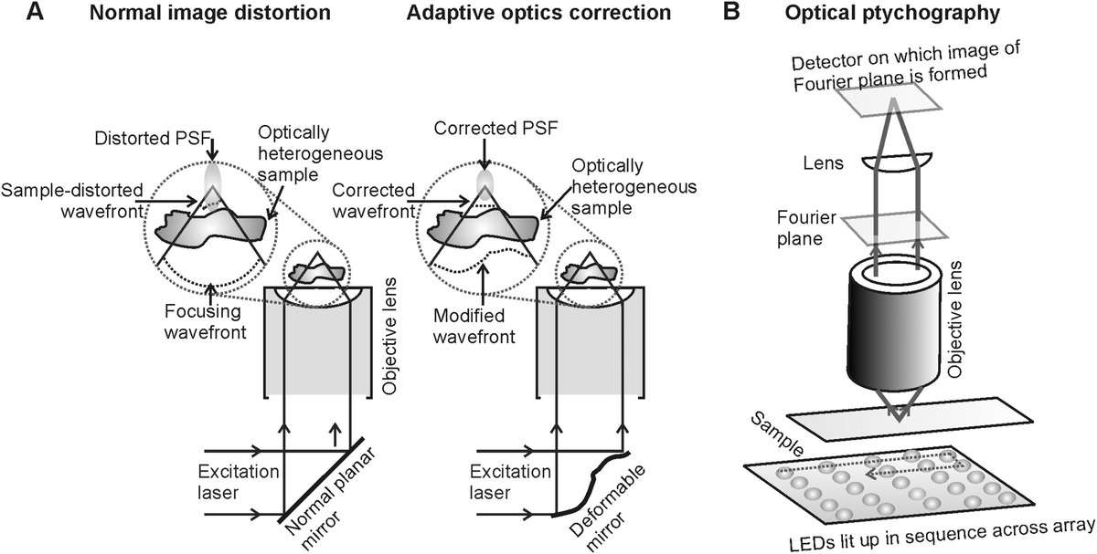
Figure 4.3 Methods to correct for image distortions and numerically refocus. (a) Uncorrected illumination (left panel) through an optically heterogeneous sample can result in image distortion during fluorescence excitation, which can be corrected by using adaptive optics (right panel, here shown with a deformable mirror on the excitation path, but a similar optical component can also be placed in the imaging path for fluorescence emissions). (b) Optical ptychography generates sample images by Fourier transforming the Fourier plane image of the sample, which permits a greater effective numerical aperture for imaging compared to the physical objective lens and also enabling numerical refocusing of the sample.
The end result is a reflattened, corrected wave front emerging from the sample (for a recent review, see Booth, 2014). AO has been applied to image to tissue depths of up to several hundred microns. It is also compatible with several different forms of light microscopy imaging techniques.
4.5.3 Ptychography Methods for Numerical Focusing
Another emerging light microscopy technique that shows promise for imaging at tissue depths in excess of 100 μm is ptychography (also referred to as Fourier ptychography). Ptychography is a label-free method, which uses advanced computational algorithms to numerically focus a sample, in effect using a virtual objective lens, and has been applied to investigating various aspects of cell cycle changes (see Marrison et al., 2013).
Ptychography was originally developed for the analysis of x-ray microscopy scattering data (see Chapter 5). With x-rays, there is no equivalent “lens” to form an image, but ptychography was implemented to allow numerical focusing from computational reconstructions of the x-ray diffraction pattern. These methods have now been implemented in light microscopy systems.
In a common design, the specimen and a coherent illuminating beam are moved relative to one another to sequentially illuminate the sample with overlapping areas (Figure 4.3b). Another method achieves a similar effect but using a 2D array of LED light sources to sequentially illuminate the sample, which circumvents the requirement for relatively slow scanning. The diffracted light pattern is then detected by a 2D pixel photodetector array, such as simple CCD camera. The spatial extent of this detector array can give access to a far greater region of reciprocal (i.e., frequency) space than is available to a physical objective lens, which is limited by its numerical aperture.
By utilizing different sequences of illumination areas, different conventional contrast enhancement modes of light microscopy can be replicated. For example, illumination in the center of the sample produces brightfield images, whereas illuminating the outer regions (equivalent to obtaining data from higher diffraction angles than those in principle obtainable from the finite small numerical aperture of a typical objective lens) can generate equivalent dark-field images. Similarly, sequentially taking pairs of images with alternating halves of the sample illuminated allows the reconstruction of phase contrast images. Performing a full sequential illumination scan over the whole extent of the sample allows accurate recovery of the phase of the wave as it travels through the specimen. This has great potential for rectifying the aberration due to optical inhomogeneity in thick samples, since corrections for the phase variations can be made numerically in reciprocal space.
One potential problem is that the detected diffraction pattern consists of just intensity data and does not contain information concerning the relative phase of a scattered beam from a particular part of the sample. However, this phase information can be recovered since the illuminated area moves over the sample to generate redundancy in the data since there is always some overlap in the sampled regions, which can be used to retrieve the phase from the scattered object using an algorithm called the “pytchographic iterative engine” (Faulkner and Rodenburg, 2004).
The main issues with ptychography are the huge volumes of data captured (a gigapixel image for each illuminated area on the sample) and a requirement for potentially very long acquisition time scales. A typical single dataset from a static biological sample contains hundreds of images to obtain sufficient information from different diffraction angles. The LED array approach improves the time resolution issue to some extent; however, to monitor any time-resolved process potentially involves datasets that would fill a normal computer hard drive very quickly.
4.5.4 Multiphoton Excitation
Multiphoton excitation (MPE) is a nonlinear optical effect. In MPE microscopy, the transition energy required to excite a ground state electron to a higher level during fluorescence excitation in a fluorophore can in principle be contributed from the summation of the equivalent quantum energies of several photons, provided these photons are all absorbed within a suitably narrow time window. In two-photon excitation microscopy (or 2PE microscopy), the initial excitation of a ground state electron is made following the absorption of two photons of the same wavelength λ during a time window of only ~10−18 s, since this is the lifetime of a virtual state halfway between the excited and ground states (Figure 4.4a). This means that λ is twice that of the required for the equivalent single-photon excitation process, and so for visible light, two-photon excitation fluorescence detection near IR (NIR) incident wavelengths (~ a micron) are typically used.
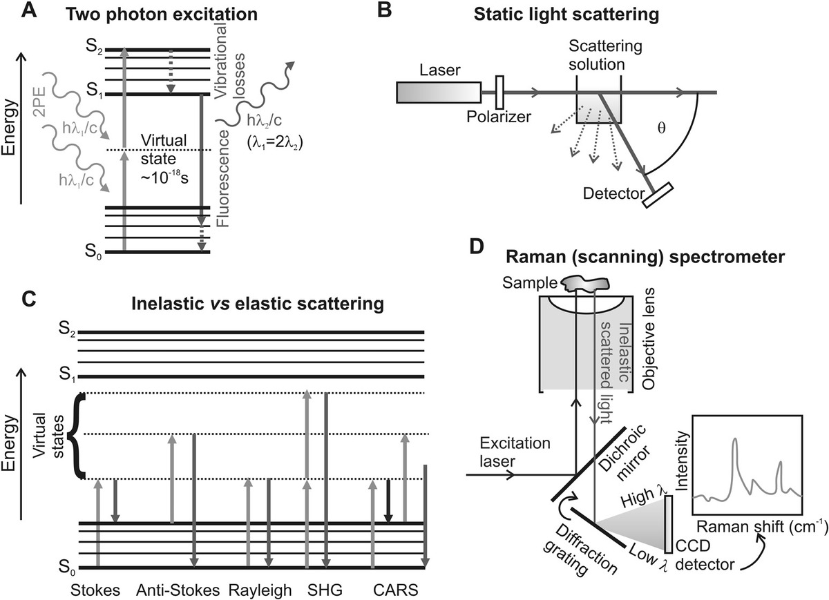
Figure 4.4 Nonlinear excitation and inelastic scattering: (a) Jablonski diagram for two-photon excitation. (b) Schematic of static light scattering apparatus. (c) Jablonski diagram for several inelastic light scattering modes compared against elastic Rayleigh scattering. (d) Schematic of Raman imaging spectrophotometer (typically based on a scanning confocal microscope core design).
Two-photon absorption, also known as the Kerr effect, is described as a third-order nonlinear effect because of the dependence of the complex polarization parameter of the optical medium on the cubic term of the electrical susceptibility. Since two photons are required, the rate of two-photon absorption at a depth z depends on the square of the incident photon intensity I, whereas for one-photon absorption, the dependence is linear, such that the overall rate has a quadratic dependence:
(4.20)where α and β are the one- and two-photon absorption coefficients, respectively.
The longer wavelengths required result is less scattering from biological tissue, for example, Rayleigh scattering, for which the length scale of the scattering objects is much smaller than the incident wavelength, has a very sensitive 1/λ4 dependence. Much of the scattering in tissue is also due to Mie scattering, that is, from objects of size comparable to or greater than λ, for which there is a less sensitive dependence of λ than for Rayleigh scattering, but still a reduction at higher wavelengths. This is significant since at depths greater than a few hundred microns, tissues are essentially opaque at visible light wavelengths due to scattering, whereas they are still optically transparent at the NIR wavelength used in two-photon microscopy. The geometrical scattering regime applies to scattering objects whose effective radius r is at least an order of magnitude greater than the wavelength of light.
The measure of the ability of an object to scatter can be characterized by its scattering cross-section. The cross-section σ can be deduced from the Mie scattering model for any general wavelength though it has a complex formulation, but the two extremes of this at very short (Rayleigh) and very high (geometrical) wavelength generate the following approximations, first for Rayleigh, σR,
(4.21)and for geometrical scattering, σG,
(4.22)where nr is the ratio of refractive indices for the scattering particle and its surrounding media, nb/nw, where nb is the refractive index of the biological scattering object and nw is the refractive index of water. In other words, the cross-section for Rayleigh scatterers scale with ~V 2 where V is their volume, whereas for geometrical scatterers this dependence with volume is much less sensitive at ~V2/3.
Another advantage of two-photon microscopy is the greater localization precision of the excitation volume. The effective cross-section for two-photon absorption is very small compared to the single-photon absorption process due to the narrow time window required for the absorption process. This requires a high incident flux of photons from a focused laser source with the two-photon absorption only probably very close to the center of the focal volume. This means that the effective focal excitation volume is an order of magnitude smaller than that of single-photon confocal microscopy, or ~0.1 fl. Thus, the excitation is significantly more localized, resulting in far less contamination in the images from out of focal plane emissions.
The spectral emission peak of QDs is temperature sensitive since the population of high-energy excitons is governed by the Boltzmann factor, which is temperature sensitive, but this sensitivity is significantly more for two-photon laser excitation compared to the standard one-photon excitation process (see Chapter 3), and this has been exploited in using QDs as nanother-mometers (see Maestro et al., 2010). This is manifest as a drop in QD brightness when measuring over a wavelength window close to the peak of a factor of ~2 when changing the local temperature from 30°C to 50°C and thus potentially is a good probe for investigating temperature changes relevant to biological samples, which has been tested as a proof-of-principle to measure the local temperatures inside human cancer cells.
A significant disadvantage with 2PE microscopy is that the incident light intensity needs to be so high that photodamage/phototoxicity becomes problematic; this can be seen clearly by using death sensors, in the form of individual muscle cells whose speed of contraction is inversely proportional to the extent of their photodamage. Also, the technique requires raster scanning technology before images can be reconstructed, and so it is slower than camera detector pixel array–based imaging, which requires no scanning, limiting the range of dynamic biological processes that can be investigated. However, tissue depths of up to 1.6 mm have been imaged using 2PE, with investigation of gray brain matter in mice (Kobat, 2011).
The limit beyond this depth using 2PE is again due to scatter resulting from unavoidable single-photon scattering. To counteract this, researchers have developed three-photon excitation microscopy, such that the wavelength of the incident photons is three times that of the required for the equivalent single-photon absorption event, which reduces the single-photon scattering even more. 3PE has enabled brain imaging in mice to be extended to ~2.5 mm depth (Horton et al., 2013).
Developments in optogenetics technologies (Chapter 7) have also benefited from MPE microscopy. Optogenetics is a method that uses light to control nerve tissue by genetically inserting lightsensitive proteins into nerve cells that open or close ion channels in response to the absorption of light at specific wavelengths. In combining this approach with 2PE, it is now possible to control the operation of multiple specific nerve fibers relatively deep in living tissue (Prakash et al., 2012).
4.5.5 Second-Harmonic Imaging
While conventional light microscopes obtain image contrast largely from the spatial differences either in optical density or refractive index in the sample, second-harmonic imaging (SHI) microscopy utilizes the generation of second harmonics from the incident light in the sample. Second-harmonic generation (SHG), or frequency doubling, involves two photons of the same frequency interacting to generate a single photon with twice the frequency and half the wavelength (an example of sum frequency generation). Biological matter capable of SHG requires periodic structural features with chiral molecular components, which result in birefringence, an optical feature in which the refractive index of a medium depends upon the wavelength of incident light (see Chapter 3). Good examples of this are the extracellular matrix protein collagen, well-ordered myosin protein filaments in muscle tissue, microtubules from the cytoskeleton, and structurally ordered features of cell membranes. SHI can also be used in monitoring the formation of crystals (see Chapter 7) for use in x-ray crystal diffraction, which can be used for determining the structure of biomolecules to an atomic level precision (see Chapter 5).
SHI microscopy offers many advantages for in vivo imaging. It is a label-free method and so does not impair biological function due to the presence of a potentially bulky fluorophore probe. Also, since it requires no fluorescence excitation, there is less likelihood from phototoxicity effects due to free radical formation. Typically, SHI microscopy is utilized with NIR incident light and so has much reduced scattering effects compared to visible light methods and can be used to reconstruct 3D images of deep tissue samples. Similarly, third-harmonic imaging microscopy, in which three incident photons interact with the sample to generate a single photon of one-third the original wavelength, has been utilized in some in vivo investigations (see Friedl, 2007).
4.5.6 Light Sheet Microscopy
Light sheet microscopy, also known as selective plane illumination microscopy, is a promising biophysical tool that bridges the length scales between single-cell imaging and multicellular sample imaging (see Swoger et al., 2014, for a modern review). It evolved from confocal theta microscopy and involves orthogonal-plane fluorescence optical sectioning; illuminating a sample from the side typically via a thin sheet of light was generated using a cylindrical lens onto a single plane of a transparent tissue sample, which has been fluorescently labeled. Since just one plane of the sample is illuminated, there is minimal out-of-plane fluorescence emission contamination of images, permitting high-contrast 3D reconstruction of several diverse in vivo features.
The development of live fruit fly embryos has been investigated with this technique (Huisken et al., 2004), as well as tracking of nuclei in live zebrafish embryos (Keller et al., 2008), growing roots tissue in developing plants, developing gut tissue, and monitoring down to subcellular levels in functional salivary glands to imaging depths of ~200 μm (Ritter et al., 2010). Variants of this technique have now been applied to monitor single cells.
A recent tissue decolorization method has been used on live mice in combination with light sheet fluorescence microscopy (Tainaka et al., 2014). This involves using a specific chemical treatment involving aminoalcohol, which results in removing the normal pink color associated with oxygen-carrying heme chemical groups in the hemoglobin of the red blood cells, thereby decolorizing any tissue that contains blood. Decolorization thus reduces the absorption of excitation light and improves its depth of penetration in live tissues and its consequent signal-to-noise ratio, facilitating single-cell resolution while performing whole-body imaging. This approach shows significant promise in determining the functional interactions between cells in living tissue, to the so-called cellular circuits of organisms.
4.5.7 Optical Coherence Tomography
Optical coherence tomography (OCT) is based on low-coherence interferometry. It uses the long coherence length of light sources to act as a coherence rejection filter to reduce the detection of multiple scattering events. In conventional interference techniques, for example, single-wavelength laser interferometry, interference occurs over a distance of a few meters. In OCT, a less coherent light source, for example, an LED, might be used, which exhibits shorter coherence lengths over a few tens of microns, which is useful for biophysics in corresponding approximately to the length scale of a few layers of cells in a tissue.
The incident light in an OCT system is normally divided into two beams to form a sample path and a reference path. A confocal light volume is typically used as a mode of illumination onto a sample. After both beams are scattered from the confocal volume, they are recombined and imaged onto one or more photodiode detectors. The two beams will generate an interference pattern on the detector if the optical path length from both beams is less than the coherence length of the light source.
In conventional light microscopy, the majority of scattered light generates background noise. This is especially prevalent with deep tissue imaging due to multiple scattering events through several layers of cells. However, in OCT, multiple scatter events can be rejected on the basis of them having a longer optical path length than the optical coherence length, since these events do not form an interference pattern. Thus, an accepted scattered photon will have arrived typically from just a single back reflection event from a cellular structure.
This rejection of multiple scatter noise permits a 3D tomographic image to be reconstructed down to a depth of a several tens of microns. OCT is now a standard technique in biomedical imaging for ophthalmology, for example, to generate 3D details of the retina of the eye but is emerging as a useful biophysical tool in research labs for imaging deep tissues and bacterial biofilms.
A variant of OCT is angle-resolved low-coherence interferometry (a/LCI). This is a relatively new light-scatting tool, which can obtain information about the size of cellular structures, including organelles such as cell nuclei. It combines the depth resolution of OCT with angle-resolved elastic light-scattering measurements (see section in the following text) to obtain in-depth information on the shape and optical properties of cellular organelles. In a/LCI, the light scattered by a sample at different angles is mixed with a reference beam to produce an inference pattern. This pattern can then be analyzed to generate the spatial distribution of scattering objects in the sample using inverse light-scattering analysis based on Mie scattering theory, which assumes spherical scattering objects (or the equivalent T-matrix theory, which is computationally more expensive but can be applied to nonspherical particles). Since the interference pattern is a measure of differences in optical path length of the scale of less than the wavelength of light, this approach can generate very precise estimates of the size and shape of intracellular-scattering objects like nuclei. This biophysical technology also shows promise as a clinical tool for detecting cancerous cells.
4.5.8 Removing the Deep Tissue Barrier
Arguably, the simplest approach to overcoming the issues of optical heterogeneity and signal and the attenuation effect of excitation and signal intensity of light when imaging through relatively thick sections of biological tissue is to remove that barrier of thick tissue. For example, this approach has been used in experiments on nerve cells in the brains of living rodents and primates using an optogenetics approach. To excite the proteins in individual nerve cells using light, it is often easiest to remove a small section of the bone from the skull. Superficial areas of the brain (i.e., relatively close to the skull), which include the cerebral cortex responsible for voluntary control of muscles, can then be activated by light using either an optical fiber or LED directly mounted to the skull of the animal, so that the light does not have to propagate through the bony tissue. Other methods transect out a portion of bone from the skull but replace it using a zirconium dioxide substrate (also known as zirconia), which is mechanically strong but optically transparent. Areas of the brain far from the surface can, in principle, be accessed using implanted optical fibers to deliver and receive light as appropriate.
Similar tissue resection methods can be applied for imaging several types of biological tissues that are close to the surface. Optical fibers can also be used more generally to access deeper into tissue, for example, by directing an optical fiber through natural channels in an animal whose diameter is larger than that of a cladded optical fiber. A multimodal cladded fiber has a diameter of a few hundred microns, which is small enough to be directed through the gut, large blood vessels, and lymphatic vessels. This at least allows the light source/detector to be brought close enough to the internal surface of many organs in the body within significant disruption to the native physiology.
4.6 Advanced Biophysical Techniques Using Elastic Light Scattering
Scattering of light, as with all electromagnetic or matter waves, through biological matter is primarily due to linear optical processes of two types, either elastic or inelastic. Rayleigh and Mie/Tyndall scattering (see Chapter 3) are elastic processes in which an emergent scattered photon has the same wavelength as the incident photon. In the previous chapter, we encountered Mie/Tyndall scattering used in simple optical density measurements in a visible light spectrophotometer to determine the concentration of scattering particles such as cells in a sample. More advanced applications of elastic light scattering, which can reveal molecular level details, include specific techniques called “static light scattering” (SLS) and “dynamic light scattering” (DLS).
Rayleigh scattering occurs when the scattering particle has a length scale at least an order of magnitude less than the incident light (a semiarbitrary condition often used is that the length scale is less than ~1/20 of the light wavelength), such that the entire surface of the particle will in effect scatter roughly with the same phase. This is the length scale regime of many small biomolecules and molecular complexes. If molecules are randomly positioned, the arrival of a photon at any molecular surface will be random, resulting in incoherent scattered light whose intensity is just the sum of squares of the amplitudes from all particles. Using a simple harmonic dipole oscillator model for electromagnetic radiation scattering leads to the Rayleigh equation (or scattering formula):
(4.23)where IS is the Rayleigh scattered light of wavelength λ when measured at a distance d and angle θ from the incident light direction from a sample composed of C scattering particles per unit volume of refractive index n and effective radius r. Thus, the scattered intensity is proportional to the reciprocal of the fourth power of the light wavelength and the sixth power of its radius.
4.6.1 Static Light Scattering
SLS can be used to obtain estimates for the molecular weight Mw of an in vitro biological sample in the Rayleigh scattering regime, and for larger molecules in the Mie scattering regime can estimate Mw as well as generate a measure of the length scale of such macromolecules given by their root-mean-squared radius, denoted as the radius of gyration, RG.
Typically, the scattered intensity from a visible laser light beam incident on an in vitro solution of a particular type of biomolecule at high concentration (equivalent to ~1 mg mL−1), or a mixture of molecule types, is measured as a function of the scatter angle θ (Figure 4.4b), either by rotating the same detector or by using multiple fixed detectors located at different angles (multiangle light scattering), often using 10 different values of θ spanning a typical range ~30°–120°. A time-averaged scattered signal intensity is obtained at each angle; hence, there is no time-resolved information and so the technique is described as “static.”
One analytical approach to understand these data is to apply continuum modeling (i.e., to derive an analytical formulation) to Rayleigh scattering (which is clearly from discrete particles) to approximate the scattering as emerging from scattering centers that are local fluctuations δC in the continuum concentration function for molecules in solution. This fluctuation approach is a common theoretical biophysical tool used to interface continuum and discrete mathematical regimes (see Chapter 8). Here, δC can be estimated from the Boltzmann distribution through a fluctuation in chemical potential energy Δμ, which relates to the osmotic pressure of the solution Π in the sample volume V, through a simple Taylor expansion of the natural logarithm of (1 − δC), as
(4.24)where
- R is the molar gas constant
- T is the absolute temperature
But Π can also be related to C through a virial expansion that is in essence an adaptation of the ideal gas law but taking into account real effects of interaction forces between molecules and the solvent (usually an organic solvent such as toluene or benzene). This indicates
(4.25)where B is the second virial coefficient. Combining Equations 4.23 through 4.25 gives the Debye equation:
(4.26)where R is the Rayleigh ratio given by:
(4.27)And the factor K depends on the parameters of the SLS instrument and the molecular solution:
(4.28)Therefore, a linear plot of KC/R versus C has its intercept at 1/Mw. Thus, Mw can be determined.
For larger molecules in the Mie/Tyndall scattering regime, the Debye equation can be modified to introduce a form or shape factor P(Q), where Q is the magnitude of scattering vector (the change in the photon wave vector upon scattering with matter):
(4.29)The exact formulation of P depends on the 3D shape and extension of the molecule, embodied in the RG parameter. The most general approximation is called the “Guinier model,” which can calculate RG from any shape. A specific application of the Guinier model is the Zimm model that assumes that each molecule in solution is approximated as a long random coil whose end-to-end length distribution is dependent on a Gaussian probability function, a Gaussian polymer coil (see Chapter 8), and can be used to approximate P for relatively small Q:
(4.30)The scattering vector in the case of elastic scattering can be calculated precisely as
(4.31)Therefore, a plot of KC/R versus C at high values of θ would have a gradient approaching ~2B, which would allow the second virial coefficient to be estimated. Similarly, the gradient at small values of θ approaches
A mixed/polydisperse population of different types of molecules can also be monitored using SLS. The results of Mw and RG estimates from SLS will be manifested with either multimodal distributions or apparent large widths to unimodal distributions (which hides underlying multimodality). This can be characterized by comparison with definitively pure samples. The technique is commonly applied as a purity check in advance of other more involved biophysical techniques, which require ultrahigh purity of samples, for example, the formation of crystals for use in x-ray crystallography (see Chapter 7).
4.6.2 Dynamic Light Scattering
Dynamic light scattering (DLS), also referred to as photon correlation spectroscopy (or quasielastic light scattering), is a complementary technique to SLS, which uses the time-resolved fluctuations of scattered intensity signals, and is therefore described as “dynamic.” These fluctuations result from molecular diffusion, which is dependent on molecular size. It can therefore be used to determine the characteristic hydrodynamic radius, also known as the Stokes radius RS, using an in vitro solution of biomolecules, as well as estimating the distribution of the molecular sizes in a polydisperse solution.
As incident light is scattered from diffusing biomolecules in solution, the motion results in randomizing the phase of the scattered light. Therefore, the scattered light from a population of molecules will interfere, both destructively and constructively, leading to fluctuations in measured intensity at a given scatter angle θ as a function of time t. Fluctuations are usually quantified by a normalized second-order autocorrelation function g, similar to the analysis performed in FCS discussed previously in this chapter:
(4.32)A monodispersed molecular solution can be modeled as gm:
(4.33)where gm(∞, θ) is the baseline of the autocorrelation function at “infinite” time delay. In practice, autocorrelations are performed using time delays τ in the range ~10−6 s−1, and so gm(∞, θ) would be approximated as ~gm using a value of ~1 s for τ. However, in many experiments, there is often very little observable change in g at values of τ above a few milliseconds, since this is the typical diffusion time scale of a single molecule across the profile of the laser beam in the sample.
Q in Equation 4.30 is the θ-dependent scattering vector as described previously in Equation 4.28. Many conventional DLS machines monitor exclusively at a fixed angle θ = 90°; however, some modern devices allow variable θ measurement. In conventional DLS, the sample often has to be diluted down to concentration levels equivalent to ~0.l mg mL−1 to minimize stochastic noise on the autocorrelation function from scattered events through the entire sample cuvette. “Near” backscatter measurements (e.g., at θ ≈ 170°) have some advantages in that they allow focusing of the incident laser beam to sample scattered signals just from the front side of sample cuvette, which reduces the need to dilute the sample, thus increasing the total scattered intensity signal.
D is the translational diffusion coefficient for the biomolecule. This is related to the drag coefficient by the Stokes–Einstein relation (Equation 2.11), which, for a perfect sphere, is given by
(4.34)where
- kB is the Boltzmann constant
- T is the absolute temperature
- η is the viscosity of the solvent
Thus, by fitting gm to the experimental autocorrelation data, the diffusion coefficient, and hence the Stokes radius of the molecule, can be determined. A polydisperse system of N different biomolecule types generates an N-modal autocorrelation response, which can be approximated by a more general model of
(4.35)Thus, in principle, this allows estimation of the Stokes radii of several different components present in solution, though in practice separating out more than two different components in this way can be nontrivial unless they have distinctly different sizes.
4.6.3 Electrophoretic Light Scattering
A modification of DLS is electrophoretic light scattering. Here, an oscillating electric E-field is applied across the sample during DLS measurements, usually parallel to the incident laser light. This results in biased electrophoretic velocity of the molecules in solution, v, determined by the molecules electrophoretic mobility μE, which depends on their net surface charge:
(4.36)A laser beam is first split between a reference and a sample path, which are subsequently recombined to generate an interference pattern at the photodetector. The molecular motion from electrophoresis results in a Doppler shift (νD) on the distribution of fluctuation frequencies observed from the scattered signal, manifested as a phase shift between the sample and reference beams, which can therefore be measured as a change in the interference pattern at the photodetector. On simple geometrical considerations
(4.37)If we consider a molecule as an ideal sphere, and balance the electrophoretic and drag forces, this indicates that
(4.38)where γ is the viscous drag coefficient on the sphere of Stokes radius (Rs) and net surface charge q in a solution of viscosity η. Thus, the net surface charge on a molecule can be estimated as
(4.39)The Stokes radius can be estimated using similar autocorrelation analysis to that of DLS earlier. The net surface charge can be related to other useful electrical parameters of a molecule, such as the zeta potential. For biological colloidal dispersions such as large biomolecules in water, the zeta potential is the voltage difference between the water in the bulk of the bulk liquid and the electrical double layer (EDL) of ions and counterions held by electrostatic forces to the molecule surface. The EDL is an important parameter in determining the extent of aggregation between biomolecules in solution.
4.6.4 Interferometric Elastic Light Scattering for Molecular Imaging
Interferometric light scattering microscopy (a common method used is known as iSCAT) has sufficiently high contrast to enable imaging of single protein molecules without the need for any fluorescent labels, for example, demonstrated with the observation of nanoscale molecular conformational changes of the protein myosin used in the contraction of muscle tissue. Here, the sample is illuminated using coherent laser light, such that the sample consists of weakly scattering objects localized on a microscope coverslip at the glass–water interface. The detected light intensity (Id) from a fast camera detector is the sum of reflected light from this interface and that scattered from the proteins on the coverslip surface:
(4.40)where
- Ei, Eref, and Escat are the incident, reflected, and scattered light E-field amplitudes
- R and s are the reflected and scattering amplitudes
- ϕ is the phase between the scattered and reflected light
For small scattering objects, the value of |s|2 is close to zero. This is because the Rayleigh scattering cross-section, and hence the scattering amplitude |s|2, scales with V2 for a small scattering particle whose radius is much less than the wavelength of light (see Equation 4.21), for example, the scattering cross-section of a 40 nm gold nanoparticle is ~107 that of a typical globular protein of a few nanometers in effective diameter; a few tens of nanometers is the practical lower limit for reproducible detection of scattered light from the laser dark-field technique (see Chapter 3), which demonstrates the clear problem with attempting to detect the scatter signal from small biomolecules directly. However, the interference term 2R|s|sin ϕ only scales with V and so is far less sensitive to changes in scatterer size, and the detection of this term is the physical basis of iSCAT.
An iSCAT microscope setup is similar to a standard confocal microscope, in terms of generating a confocal laser illumination volume, which is laterally scanned across the sample, though instead of detecting fluorescence emissions, the interference term intensity is extracted by combining a quarter wave plate with a polarizing beamsplitter. This utilizes the phase difference between the interference term with respect to the incident illumination and rotates this phase to enable highly efficient reflection of just this component at the polarizing beamsplitter, which is directed not through a pinhole as for the case of traditional confocal microscopy but rather onto a fast CCD camera, such as a CMOS camera.
An enormous advantage of iSCAT, and similar interferometric imaging methods, over fluorescence imaging is speed. Fluorescence imaging can achieve a significant imaging contrast but to do so ultimately requires a sufficiently large sampling time window to collect fluorescence emission photons. Fluorophores, as we have seen, are ultimately limited by the number of photons that they can emit before irreversible photobleaching. Interferometric scattering is not limited in this manner; in fact, the background signal in iSCAT scales with ~√N from Poisson sampling statistics, where N is the number of scattered photons detected; therefore, since the signal scales with ~N, then the imaging contrast, which is a measure of the signal-to-noise ratio, itself scales with √N. That is, a larger contrast is achievable by simply increasing the power of laser illumination. There is no photon-related physical limit, rather a biological one in increased sample damage at high laser powers.
4.7 Tools Using the Inelastic Scattering of Light
Scattering of light, as with all electromagnetic or matter waves, through biological matter is primarily due to linear optical processes of two types, either elastic or inelastic. Rayleigh and Mie scattering (see Chapter 3) are both elastic processes in which the emergent scattered photon has the same wavelength as the incident photon. One of the key inelastic processes with regard to biophysical techniques is Raman scattering. This results in the incident photon either losing energy prior to scattering (Stokes scattering) or gaining energy (anti-Stokes scattering). For most biophysical applications, this energy shift is due to vibrational and rotational energy changes in a scattering molecule in the biological sample (Figure 4.4c), though in principle the Raman effect can also be due to interaction between the incident light and to a variety of quasiparticles in the system, for example, acoustic matter waves (phonons). There are also other useful inelastic light scattering processes that can also be applied to biophysical techniques.
4.7.1 Raman Spectroscopy
Raman scattering is actually one of the major sources of bleed-through noise in fluorescence imaging experiments, which comes mainly from anti-Stokes scattering of the incident excitation light from water molecules. A Raman peak position is normally described in terms of wavenumbers (2π/λ with typical units of cm−1), and in water, this is generally ~3400 cm−1 lower/higher than the equivalent excitation photon wavenumber depending on whether the peak is Stokes or anti-Stokes (typically higher/lower wavelengths by ~20 nm for visible light excitation).
Some dim fluorophores can have comparable Raman scatter amplitudes to the fluorescence emission peak itself (i.e., this Raman peak is then the limiting noise factor). However, in general, the Raman signal is much smaller than the fluorescence emission signal from typical fluorophores, and only 1 in ~106 incident photons will be scattered by the Raman effect. But a Raman spectrum, although weak, is a unique signature of a biomolecule with a big potential advantage over fluorescence detection in not requiring the addition of an artificial label to the biomolecule.
The Raman effect can be utilized in biophysics techniques across several regions of the electromagnetic spectrum (including x-rays, see Chapter 5), but most typically, a near IR laser (wavelength ~1 μm) is used as the source for generating the incident photons. The shift in NIR Raman scattered energy for biomolecules is typically measured in the range ~200–3500 cm−1. Lower energy scattering effects in principle occur in the range ~10–200 cm−1; however, the signal from these typically gets swamped by that due to Rayleigh scattering.
A Raman spectrometer consists of a laser, which illuminates the sample, with scattered signals detected at 90° from the incident beam (Figure 4.4d). A notch rejection filter, which attenuates the incident laser in excess of 106 over a narrow bandwidth of a few nanometers, eliminates the bulk of the elastic Rayleigh scattering component, leaving the inelastic Raman scattered light. This is imaged by a lens and then spatially split into different color components using a diffraction grating, which is projected onto a CCD detector array such that different pixel positions correspond to different wavenumber shift values. Thus, the distribution of pixel intensities corresponds to the Raman spectrum.
In principle, Raman spectroscopy has some similarities to IR spectroscopy discussed in Chapter 3. However, there are key differences to IR spectroscopy, for example, the Raman effect is scattering as opposed to absorption, and also although the Raman effect can cause a change in electrical polarizability in a given chemical bond, it does not rely on exciting a different bond vibrational mode, which has a distinctly different electrical dipole moment. Key biomolecule features that generate prominent Raman scattering signatures include many of the bonds present in nucleic acids, proteins, lipids, and many sugars. The weakness of the Raman scatter signal can be enhanced by introducing small Raman tags into specific molecular locations in a sample, for example, alkyne groups, which give a strong Raman scatter signal, though this arguably works against the primary advantage of conventional Raman spectroscopy over fluorescence-based techniques in being label-free.
4.7.2 Resonance Raman Spectroscopy
When the incident laser wavelength is close to the energy required to excite an electronic transition in the sample, then Raman resonance can occur. This can be especially useful in enhancing the normally weak Raman scattering effect. The most common method of Raman resonance enhancement as a biophysical tool involves surface-enhanced Raman spectroscopy (SERS), which can achieve molecular level sensitivity in biological samples in vitro (see Kneipp et al., 1997).
With SERS, the sample is placed in an aqueous colloid of gold or silver nanoparticles, typically a few tens of nanometers in diameter. Incident light can induce surface plasmons in the metallic particles in much the same way as they do in surface plasmon resonance (see Chapter 3). In the vicinity of the surface, the photon electric field E is enhanced by a factor ~E4. This enhancement effect depends sensitively on the size and shape of the nanoparticles. For spherical particles, the enhancement factor falls by 50% over a length scale of a few nanometers.
Heuristic power-law dependence is often used to model this behavior:
(4.41)where I(z) is the Raman scatter intensity at a distance z from surface of a spherical particle of radius R. Although different experimental studies suggest that the parameter a varies broadly in the range ~3–6, with ~4.6 being given consensus by many.
A typical enhancement in measurement sensitivity, however, is >105, with values up to ~1014 being reported. Therefore, if a biomolecule is bound to the surface of a nanoparticle, then an enhanced Raman spectrum can be generated for that molecule. The enhancement allows sample volumes of ~10−11 L to be probed at concentrations of ~10−14 M, sufficiently dilute to permit single-molecule detection (for a review, see Kneipp et al., 2010).
SERS has been applied to detecting nucleotide bases relevant to DNA/RNA sequencing, amino acids, and large protein structures such as hemoglobin, in some cases pushing the sample detection volume down to ~10−13 L. It has also been used for living cell samples, for example, to investigate the process of internalization of external particles in eukaryotic cells of endocytosis (see Chapter 2).
SERS can also be used in conjunction with microscale tips used in AFM (see Chapter 6). These tips are pyramidal in shape and have a height and base length scale of typically several microns. However, the radius of curvature is more like ~10 nm, and so if this is coated in gold or silver, there will be a similar SERS effect, referred to as tip-enhanced Raman spectroscopy (TERS), which can be used in combination with AFM imaging. Recently, carbon nanotubes have also been used as being mechanically strong, electrically conductive extensions to AFM tips.
SERS has also been performed on 2D arrays of silver holes nanofabricated to have diameters of a few hundred nanometers. The ability to controllably nanofabricate a 2D pattern of holes has advantages in increased throughput for the detection of biological particles (e.g., of a population of cells in a culture, or a solution of biomolecules), which facilitates miniaturization and coupling to microfluidics technologies for biosensing application. Also, although still in its infancy, the technology is compatible with rendering angle-resolved Raman scattering signals in using a polarized light source, which offers the potential for monitoring molecular orientation effects.
4.7.3 Raman Microscopy
A Raman microscope can perform Raman spectroscopy across a spatially extended sample to generate a spatially resolved Raman spectral image. Raman microscopy has been used to investigate several different, diverse types of cells grown in culture. For example, these include spores of certain types of bacteria, sperm cells, and cells that produce bone tissue (osteocytes). In its simplest form, a Raman microscope is a modified confocal microscope whose scattered light output captured by a high NA objective lens is then routed via an optical fiber to a Raman spectrometer. Devices typically use standard confocal microscope scanning methods.
This is an example of hyperspectral imaging or chemical imaging. In the case of Raman microscopy, it can generate thousands of individual Raman spectra across the whole of the field of view. The molecular signatures from these data can then, in principle, be extracted computationally and used to generate a 2D map showing the spatial localization and concentration of different biochemical components in cellular samples. In practice, however, it is challenging to extract the individual signature from a complex mix of anything more than a handful of different biochemical components due to the overlap between Raman scatter peaks, and so the method is largely limited to extracting strong signals from a few key biochemical components.
Hyperspectral imaging is a slow technique, limited by the scanning of the sample but also in the required integration time for a complete Raman spectrum to be generated for each pixel in the digitized confocal Raman map. A typical scan for a small pixel array can take several minutes. This increased exposure to incident light increases the risk of sample photodamage and limits the utility of the technique for monitoring dynamic biological processes.
Improvements in sampling speed can be made using direct Raman imaging. Here, only a very narrow range of wavenumbers corresponding to a small Raman scattering bandwidth is sampled to allow a standard 2D photodetector array system, such as an EMCCD camera, to be used to circumvent the requirement for mechanical scanning and full Raman spectrum acquisition, for example, to monitor the spatial localization of just a single biochemical component such as cholesterol in a cell. Also, the temporal resolution is improved using related coherent Raman spectroscopy methods. This has significant advantages for this emerging field of chemical imaging; this is an example of a biophysical imaging technique used to investigate the chemical environment of biological samples, and improving the time resolution enables better insight into the underlying dynamics of this chemistry.
4.7.4 Coherent Raman Spectroscopy Methods
Two related Raman techniques that specifically use coherent light sources are coherent anti-Stokes Raman scattering (CARS) and coherent Stokes Raman scattering (CSRS, pronounced “scissors”). However, CSRS is rarely favored over CARS in practice because its scattering output is at higher wavelengths than the incident light and is therefore more likely to be contaminated by autofluorescence emissions. CARS, in particular, has promising applications for in vivo imaging. Both CARS and Raman spectroscopy use the same Raman active vibration modes of molecular bonds, though the enhancement of the CARS signal compared to conventional Raman spectroscopy is manifested in an improvement in sampling time by a factor of ~105. In other words, CARS can be operated as a real-time video-rate technique.
CARS is a third-order nonlinear optical effect, which uses three lasers, one to pump at frequency ωpump, a Stokes laser of frequency ωStokes, and a probe laser at frequency ωprobe. All these interact with the sample to produce a coherent light output with anti-Stokes shifted frequency of (ωpump + ωprobe − ωStokes). When the frequency difference between the pump and the Stokes lasers (i.e., ωpump − ωStokes) coincides with the Raman resonance frequency of a specific vibrational mode of a molecular bond in the sample, there is a significant enhancement of the output. Molecules such as lipids and fatty acids, in particular, have strong Raman resonances. When combined with microscopic laser scanning, 2D images of in vivo samples can be reconstructed to reveal high-resolution details for cellular structures that have high fat content, a good example being the fatty myelin sheath, which acts as a dielectric insulator around nerve fibers, with some CARS imaging systems now capable of video-rate time resolution. This technology not only gives access to dynamic imaging of biochemical components in cell populations that are difficult to image using other techniques but like conventional Raman spectroscopy is also a label-free approach with consequent advantages of reduced impairment to biological functions compared to technologies that require components to be specifically labeled.
4.7.5 Brillouin Light Scattering
When light is transmitted through a sample that contains periodic variation in refractive index, Brillouin light scattering (BLS) can occur. In a biological sample, the most likely cause of Brillouin inelastic scattering is the interaction between acoustic oscillation of the sample matter, in the form of phonons, and the incident light. Phonons can establish standing waves in a sample, which causes the periodic changes to the molecular structure correlated over an extended region of the sample, resulting in periodicity in refractive index over the length scale of phonon wavelengths.
Similar to Raman scattering, an incident photon of light can gain energy from a phonon (Stokes process) or lose energy in creating a phonon in the material (anti-Stokes process), resulting in a small Brillouin shift to the scattered light’s wavelength. The shift can be quantified by a Brillouin spectrometer, which works on principles similar to a Fabry–Pérot interferometer (or etalon), as discussed in Chapter 3. Although not a unique fingerprint in the way that a Raman spectrum is, a Brillouin spectrum can render structural details of optically transparent biological materials, for example, to investigate the different optical materials in an eye. The largest technical drawbacks with Brillouin spectroscopy are the slowness of sampling and the often limited spatial information, in that most devices perform essentially point measurements, which require several minutes to acquire. However, recent developments have coupled Brillouin spectroscopy to confocal imaging to generate a Brillouin microscope, with improvements in parallelizing of scatter signal sampling to permit sampling rates of ~1 Hz per acquired spectrum (Scarcelli and Yun, 2007). BLS has been used in a number of studies to investigate the biomechanical properties of a variety of tissues, which are discussed in Chapter 6.
4.8 Summary Points
- There are several super-resolution methods, characterized by techniques that use light microscopy to determine the location of a single dye molecule better than the diffraction-determined optical resolution limit.
- An array of nonlinear methods is useful for studying biological processes deep into tissues, especially two-photon excitation fluorescence imaging.
- Tools to correct for optical inhomogeneity in deep tissues exist, such as AO.
- Interactions between two different biomolecules can be monitored using FRET, down to the level of single molecules.
- FCS is a robust tool to determine diffusion rates, which complements single-particle tracking methods.
- Inelastic scattering methods such as Raman and Brillouin scattering are “label-free” and facilitate monitoring of a range of biomolecule types beyond just the primary focus of fluorescence microscopy, which is fluorescently labeled proteins.
Questions
- 4.1 A high-power oil-immersion objective lens has an NA or 1.45, transmitting 80% of visible light, total magnification 300.
- What is the photon capture efficiency of the lens? In a TIRF experiment using the objective lens method with a laser excitation of wavelength 561 nm, a protein is labeled with the FP mCherry.
- Using PubSpectra (http://www.pubspectra.org/) or equivalent, select a suitable dichroic mirror and emission filter for exciting and visualizing mCherry molecules and estimates the maximum proportion of fluorescence photons that can in principle reach a camera detector.
- If the camera detector converts 90% of all incident visible light photons into a signal and has a pixel size of 18 μm and a background noise level (b) equivalent to ~200 counts, what is the best spatial precision with which one can estimate the position of a single mCherry molecule stuck to the surface of a glass coverslip? In an actual experiment, the best precision was measured to be approximately 10 times worse than the theoretical estimate.
- What is the most likely cause of this discrepancy?
- 4.2 Derive formulas for the relation between sigma width and w for the full width at half maximum value to a Gaussian approximation to the PSF.
- 4.3 X-ray diffraction data (see Chapter 5) suggest that a certain protein found in the cell membrane can be present as both a monomer and a dimer. A single-molecule yellow-color FP called YPet was fused to the end of this protein to perform live-cell fluorescence imaging. TIRF microscopy was used on live cells indicating typically six detected fluorescent spots of full width at half maximum intensity profile ~180 nm per cell in each illuminated section of cell membrane. TIRF microscopy here was found to illuminate only ~15% of the total extent of the cell membrane per cell, with the total membrane area being ~30 μm2 per cell. On the basis of intensity measurements of the fluorescent spots, this indicated that ~75% of the spots were monomers, ~15% were dimers, and the remaining 10% were consistent with being oligomers. Explain with reasoning if you think the oligomers are “real” or simply monomers or dimers, which are very close to each other. (Hint: if two fluorescent molecules observed using diffraction-limited microscopy are separated by less than the optical resolution limit, we may interpret them as a single “spot.”)
- 4.4 A synthetic molecular construct composed of DNA was labeled with a bright organic “intercalating” PALM dye, which decorated the DNA by binding between every other nucleotide base pair. Each organic dye molecule, once stochastically activated during PALM imaging, could fluorescently emit an average of ~107 photons of peak wavelength at ~550 nm, before irreversibly photobleaching, and could emit these at a maximum flux rate of ~108 photons per second. If the total detection efficiency for all photons emitted is 10% at the EMCCD camera of the PALM imaging device, calculate, stating any assumptions you make, what the maximum theoretical imaging frame rate on the PALM imaging device would be to permit two neighboring dye molecules on the DNA to be resolved in the focal plane of the microscope.
- 4.5 The PALM imaging device of Question 4.4 was modified to permit 3D localization of the organic dye using astigmatism imaging. If the DNA construct was aligned with the optic axis, what then is the maximum frame rate that would permit two neighboring dye molecules on the DNA to be resolved?
- 4.6 An in vitro fluorescence imaging experiment involving GFP was performed with and without the presence of the G/GOD/CAT free radical quencher. When performed in pure water without any quencher the GFP bleached rapidly, whereas upon adding the quencher the rate of bleaching was lower. If the same experiment was performed with the quencher but in a solution of PBS (phosphate-buffered saline, a simple pH buffer) the rate of bleaching was the same, but the brightness of single GFP molecules appeared to be greater than before. Explain these observations.
- 4.7 A protein is labeled with a donor and acceptor fluorophore to study a conformational change from state 1 to 2 by using single-molecule FRET. The FRET acceptor–donor pair has a known Förster radius of 4.9 nm, and the measured fluorescence lifetimes of the isolated donor and the acceptor fluorophores are 2.8 and 0.9 ns, respectively.
- Show that the FRET efficiency is given by (1 − τDA/τD) where τDA and τD are the fluorescence lifetimes of the donor in the presence and absence of acceptor, respectively.
- What is the distance between the donor and acceptor if the measured donor lifetime in conformation 1 is 38 ps? Structural data from x-ray crystallography (see Chapter 5) suggest that the fluorophore separation may increase in a distinct step by 12 Å when the protein makes a transition between states 1 and 2.
- Calculate the donor fluorescence lifetime of conformation 2. How small does the measurement error of the FRET efficiency need to be to experimentally observe? See the changes of state from 1 to 2.
- What is the maximum change in FRET efficiency that could be measured here?
- 4.8 A FLIM–FRET experiment using GFP and mCherry FPs as the donor and acceptor FRET fluorophores, respectively, indicated that the fluorescence lifetimes of both proteins were 5 ns or less. Both proteins have a molecular weight of ~28 kDa and an effective diameter of ~3 nm.
- What, with reasoning, is the typical rotational time scale of these FPs if their motions are unconstrained? The researchers performing the experiment assumed that any dynamic changes observed in the estimated FRET efficiency were due to relative separation changes of the GFP and mCherry.
- Discuss, with reasoning, if this is valid or not.
- Why is this experiment technically challenging when attempted at the single-molecule level?
- 4.9 A 4π microscope was composed of two matched oil-immersion (refractive index ≈ 1.52) objective lenses of NA 1.49. In an exam answer, a student suggested that this should be better described as a 3.2π microscope. Discuss.
- 4.10
A bespoke STED microscope used a white-light laser emitting at wavelengths from ~450 to 2000 nm of total power 6 W, generated in regular pulse bursts at a frequency of 60 MHz such that in each cycle, the laser produces a square-wave pulse of 10 ps duration.
- What is the mean power density in mW per nm from the laser?
- How does this compare with the peak power output? The excitation laser was split by a dichroic mirror and filtered to generate a blue beam that would transmit 90% of light over a 20 nm range centered on 488 nm wavelength, and zero elsewhere, before being attenuated by an ND1 filter and focused by a high NA objective lens onto a sample over an area equivalent to a diffraction-limited circle of effective diameter equal to the PSF width. A red beam was directed through a loss-free prism that would select wavelengths over a range 600–680 nm, before being attenuated by an ND4 filter, phase modified to generate a donut shape and focused by the same objective lens in the sample of area ~0.1 μm2. The oil-immersion objective lens had an NA of 1.49 and a mean visible light transmittance of 80%. A biological sample in the STED microscope consisted of fibers composed of microtubules (see Chapter 2) or diameter 24 nm, which were labeled on each tubulin monomer subunit with a fluorescent STED dye. Assume here that the saturating intensity of STED is given by the mean in the ring of the donut.
- Discuss, with reasoning, if this microscope can help to address the question of whether fibers in the sample consist of more than one individual microtubule.
- 4.11 A typical FCS experiment is performed for a single type of protein molecule labeled by GFP, which exhibits Brownian diffusion through a confocal laser excitation volume generated by focusing a 473 nm laser into the sample solution to generate a diffraction-limited intensity distribution.
- Show, stating any assumptions you make, that the number density autocorrelation function is given by
- The effective confocal volume V can be defined as
- In one experiment, the autocorrelation function at small time interval values converged to ~2.6 and dropped to ~50% of this level at a time interval value of ~8 ms. Estimate with reason the diffusion coefficient of the protein and the number of protein molecules that would be present in a 1 μL drop of that solution.
- Show, stating any assumptions you make, that the number density autocorrelation function is given by
- 4.12 A protein is labeled with a donor–acceptor FRET pair whose Förster radius is 5.1 nm to investigate a molecular conformational change from state I to II. The fluorescence lifetimes of the donor and the acceptor fluorophores are known to be 5.3 and 1.1 ns, respectively.
- The donor lifetime for state I has a measured value of 54 ps. Calculate the FRET efficiency in this state and the distance between the FRET dye pair.
- There is a decrease in this distance of 0.9 nm due to the conformational change of state I–II. Estimate the fluorescence lifetime of the donor in this state, and comment on what the error of the FRET efficiency measurement must be below in order to observe this distance change.
- 4.13 A gold-coated AFM tip was used as a fluorescence excitation source for TERS by focusing a laser beam on to the tip and then scanning the tip over a fluorescently labeled sample. The fluorescence intensity measured from the sample when the tip was close to the surface was ~106 counts, which decreased to only ~102 counts when the tip was moved back from the sample by just 1 nm. Estimate the radius of curvature of the AFM tip.
- 4.14 If a 50 nm diameter nanobead can just be detected using laser dark-field, which relies on Rayleigh scattering, with a maximum sampling frequency of 1 kHz, estimate the minimum time scale of a biological process that could in principle be investigated using the same instrument but to monitor a biomolecular complex of effective diameter of 10 nm, assuming the nanobead and biomolecules have similar refractive indices.
References
Key Reference
- Thompson, R.E., Larson, D.R., and Webb, W. (2002). Precise nanometer localization analysis for individual fluorescent probes. Biophys. J. 82:2775.
More Niche References
- Appelhans, T. et al. (2012). Nanoscale organization of mitochondrial microcompartments revealed by combining tracking and localization microscopy. Nano Lett. 12:610–616.
- Badieirostami, M. et al. (2010). Three-dimensional localization precision of the double-helix point spread function versus astigmatism and biplane. Appl. Phys. Lett. 97:161103.
- Balzarotti, F. et al. (2016) Nanometer resolution imaging and tracking of fluorescent molecules with minimal photon fluxes. Science 355:606–612.
- Benitez, J.J., Keller, A.M., and Chen, P. (2002). Nanovesicle trapping for studying weak protein interactions by single-molecule FRET. Methods Enzymol. 472:41–60.
- Betzig, E. et al. (2006). Imaging intracellular fluorescent proteins at nanometer resolution. Science 313:1642–1645.
- Booth, M. (2014). Adaptive optical microscopy: The ongoing quest for a perfect image. Sci. Appl. 3:e165.
- Broxton, M. et al. (2013). Wave optics theory and 3-D deconvolution for the light field microscope. Opt. Exp. 21:25418–25439.
- Burnette, D.T. et al. (2011). Bleaching/blinking assisted localization microscopy for superresolution imaging using standard fluorescent molecules. Proc. Natl. Acad. Sci. USA 108:21081–21086.
- Chiantia, S., Kahya, N., and Schwille, P. (2007). Raft domain reorganization driven by short- and long-chain ceramide: A combined AFM and FCS study. Langmuir 23:7659–7665.
- Churchman, L.S. et al. (2005). Single molecule high-resolution colocalization of Cy3 and Cy5 attached to macromolecules measures intramolecular distances through time. Proc. Natl. Acad. Sci. USA 102:1419–1423.
- Cissé, I. I. et al. (2013). Real-time dynamics of RNA polymerase II clustering in live human cells. Science. 341:664–667.
- Cox, S. et al. (2012). Bayesian localization microscopy reveals nanoscale podosome dynamics. Nat. Methods 9:195–200.
- Dertinger, T. et al. (2009). 3D super-resolution optical fluctuation imaging (SOFI). Proc. Natl. Acad. Sci. USA 106:22287–22292.
- Faulkner, H.M. and Rodenburg, J.M. (2004). A phase retrieval algorithm for shifting illumination. Appl. Phys. Lett. 85:4795–4797.
- Friedl, P. et al. (2007). Biological second and third harmonic generation microscopy. Curr. Protoc. Cell Biol. 4:Unit 4.15.
- Gordon, M.P., Ha, T., and Selvin, P.R. (2004). Single-molecule high-resolution imaging with photobleaching. Proc. Natl. Acad. Sci. USA 101:6462–6465.
- Gustafsson, M.G. (2000). Surpassing the lateral resolution limit by a factor of two using structured illumination microscopy. J. Microsc. 198:82–87.
- Ha, T. and Tinnefeld, P. (2012). Photophysics of fluorescence probes for single molecule biophysics and super-resolution imaging. Annu. Rev. Phys. Chem. 63:595–617.
- Ha, T. et al. (1996). Probing the interaction between two single molecules: Fluorescence resonance energy transfer between a single donor and a single acceptor. Proc. Natl. Acad. Sci. USA 93:6264–6268.
- Ha, T. et al. (2002). Initiation and re-initiation of DNA unwinding by the Escherichia coli Rep helicase. Nature 419:638–641.
- Hecht, B. et al. (2000). Scanning near-field optical microscopy with aperture probes: Fundamentals and applications. J. Chem. Phys. 112:7761–7774.
- Hell, S.W. and Stelzer, E.H.K. (1992). Fundamental improvement of resolution with a 4Pi-confocal fluorescence microscope using two-photon excitation. Opt. Commun. 93:277–282.
- Hell, S.W. and Wichmann, J. (1994). Breaking the diffraction resolution limit by stimulated emission: Stimulated-emission-depletion fluorescence microscopy. Opt. Lett. 19:780–782.
- Horton, N.G. et al. (2013). In vivo three-photon microscopy of subcortical structures within an intact mouse brain. Nat. Photon. 7:205–209.
- Huisken, J. et al. (2004). Optical sectioning deep inside live embryos by selective plane illumination microscopy. Science 305:1007–1009.
- Jones, S.A. et al. (2011). Fast, three-dimensional super-resolution imaging of live cells. Nat. Methods 8:499–508.
- Kapanidis, A.N. et al. (2005). Alternating-laser excitation of single molecules. Acc. Chem. Res. 38:523–533.
- Keller, P.J. et al. (2008). Reconstruction of zebrafish early embryonic development by scanned light sheet microscopy. Science 322:1065–1069.
- Kneipp, K. et al. (1997). Single molecule detection using surface-enhanced Raman scattering (SERS). Phys. Rev. Lett. 56:1667–1670.
- Kneipp, J. et al. (2010). Novel optical nanosensors for probing and imaging live cells. Nanomed. Nanotechnol. Biol. Med. 6:214–226.
- Kobat, D. et al. (2011). In vivo two-photon microscopy to 1.6-mm depth in mouse cortex. J. Biomed. Opt. 16:106014.
- Lee, S.F. et al. (2011). Super-resolution imaging of the nucleoid-associated protein HU in Caulobacter crescentus. Biophys. J. 100:L31–L33.
- Levoy, M. et al. (2009). Recording and controlling the 4D light field in a microscope using microlens arrays. J. Microsc. 235:144–162.
- Lew, M.D. et al. (2011). Three-dimensional superresolution colocalization of intracellular protein superstructures and the cell surface in live Caulobacter crescentus. Proc. Natl. Acad. Sci. USA 108:E1102–E1110.
- Maestro, L.M. et al. (2010). CdSe quantum dots for two-photon fluorescence thermal imaging. Nano Letters 10:5109–5115.
- Magde, D., Elson, E.L., and Webb, W.W. (1972). Thermodynamic fluctuations in a reacting system: Measurement by fluorescence correlation spectroscopy. Phys. Rev. Lett. 29:705–708.
- Marrison, J. et al. (2013). Ptychography—A label free, high-contrast imaging technique for live cells using quantitative phase information. Sci. Rep. 3:2369.
- Miyawaki, A. et al. (1997). Fluorescent indicators for Ca2+ based on green fluorescent proteins and calmodulin. Nature 388:882–887.
- Monod, J. (1971). Chance and Necessity. Vintage Books, New York.
- Mortensen, K.I. et al. (2010). Optimized localization analysis for single-molecule tracking and super-resolution microscopy. Nat. Methods 7:377–381.
- Park, H., Toprak, E., and Selvin, P.R. (2007). Single-molecule fluorescence to study molecular motors. Quart. Rev. Biophys. 40:87–111.
- Prakash, R. et al. (2012). Two-photon optogenetic toolbox for fast inhibition, excitation and bistable modulation. Nat. Methods 9:1171–1179.
- Qu, X., Wu, D., Mets, L., and Scherer, N.F. (2004). Nanometer-localized multiple single-molecule fluorescence microscopy. Proc. Natl. Acad. Sci. USA 101:11298–11303.
- Ritter, J.G. et al. (2010). Light sheet microscopy for single molecule tracking in living tissue. PLoS One 5:e11639.
- Roy, R., Hohng, S., and Ha, T. (2008). A practical guide to single-molecule FRET. Nat. Methods 5:507–516.
- Rust, M.J., Bates, M., and Zhuang, X. (2006). Sub-diffraction-limit imaging by stochastic optical reconstruction microscopy (STORM). Nat. Methods 3:793–795.
- Scarcelli, G. and Yun, S.H. (2007). Confocal Brillouin microscopy for three-dimensional mechanical imaging. Nat. Photon. 2:39–43.
- Schoen, I. et al. (2011). Binding-activated localization microscopy of DNA structures. Nano Letters 11:4008–4011.
- Swoger, J. et al. (2014). Light sheet-based fluorescence microscopy for three-dimensional imaging of biological samples. Cold Spring Harb. Protoc. 2014:1–8. http://www.nature.com/nmeth/collections/lightsheet-microscopy/index.html.
- Tainaka, K. et al. (2014). Whole-body imaging with single-cell resolution by tissue decolarization. Cell 159:911–924.
- Vollmer, F. and Arnold, S. (2008). Whispering-gallery-mode biosensing: Label-free detection down to single molecules. Nat. Methods 5:591–596.
- Warshaw, D.M. et al. (2005). Differential labeling of myosin V heads with quantum dots allows direct visualization of hand-over-hand processivity. Biophys. J. 88:L30–L32.
- Waterman-Storer, C.M. et al. (1998). Fluorescent speckle microscopy, a method to visualize the dynamics of protein assemblies in living cells. Curr. Biol. 8:1227–1230.